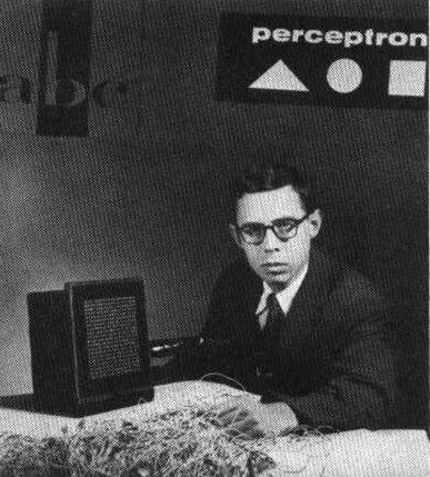
One of the first attempts to implement something similar to a modern neural network was done by Frank Rosenblatt from Cornell Aeronautical Laboratory in 1957. It was a hardware implementation called "Mark-1", designed to recognize primitive geometric figures, such as triangles, squares and circles.
 |
 |
Images from Wikipedia
An input image was represented by 20x20 photocell array, so the neural network had 400 inputs and one binary output. A simple network contained one neuron, also called a threshold logic unit. Neural network weights acted like potentiometers that required manual adjustment during the training phase.
✅ A potentiometer is a device that allows the user to adjust the resistance of a circuit.
The New York Times wrote about perceptron at that time: the embryo of an electronic computer that [the Navy] expects will be able to walk, talk, see, write, reproduce itself and be conscious of its existence.
Suppose we have N features in our model, in which case the input vector would be a vector of size N. A perceptron is a binary classification model, i.e. it can distinguish between two classes of input data. We will assume that for each input vector x the output of our perceptron would be either +1 or -1, depending on the class. The output will be computed using the formula:
y(x) = f(wTx)
where f is a step activation function
To train a perceptron we need to find a weights vector w that classifies most of the values correctly, i.e. results in the smallest error. This error is defined by perceptron criterion in the following manner:
E(w) = -∑wTxiti
where:
- the sum is taken on those training data points i that result in the wrong classification
- xi is the input data, and ti is either -1 or +1 for negative and positive examples accordingly.
This criteria is considered as a function of weights w, and we need to minimize it. Often, a method called gradient descent is used, in which we start with some initial weights w(0), and then at each step update the weights according to the formula:
w(t+1) = w(t) - η∇E(w)
Here η is the so-called learning rate, and ∇E(w) denotes the gradient of E. After we calculate the gradient, we end up with
w(t+1) = w(t) + ∑ηxiti
The algorithm in Python looks like this:
def train(positive_examples, negative_examples, num_iterations = 100, eta = 1):

    weights = [0,0,0] # Initialize weights (almost randomly :)

    for i in range(num_iterations):
        pos = random.choice(positive_examples)
        neg = random.choice(negative_examples)

        z = np.dot(pos, weights) # compute perceptron output
        if z < 0: # positive example classified as negative
            weights = weights + eta*weights.shape

        z  = np.dot(neg, weights)
        if z >= 0: # negative example classified as positive
            weights = weights - eta*weights.shape

return weightsIn this lesson, you learned about a perceptron, which is a binary classification model, and how to train it by using a weights vector.
If you'd like to try to build your own perceptron, try this lab on Microsoft Learn which uses the Azure ML designer.
To see how we can use perceptron to solve a toy problem as well as real-life problems, and to continue learning - go to Perceptron notebook.
Here's an interesting article about perceptrons as well.
In this lesson, we have implemented a perceptron for binary classification task, and we have used it to classify between two handwritten digits. In this lab, you are asked to solve the problem of digit classification entirely, i.e. determine which digit is most likely to correspond to a given image.
