


Abstract
Direct photometric measurements of the cosmic optical background (COB) provide an important point of comparison to both other measurement methodologies and models of cosmic structure formation, and permit a cosmic consistency test with the potential to reveal additional diffuse sources of emission. The COB has been challenging to measure from Earth due to the difficulty of isolating it from the diffuse light scattered from interplanetary dust in our solar system. We present a measurement of the COB using data taken by the Long-Range Reconnaissance Imager on NASA's New Horizons mission, considering all data acquired to 47 au. We employ a blind methodology where our analysis choices are developed against a subset of the full data set, which is then unblinded. Dark current and other instrumental systematics are accounted for, including a number of sources of scattered light. We fully characterize and remove structured and diffuse astrophysical foregrounds including bright stars, the integrated starlight from faint unresolved sources, and diffuse galactic light. For the full data set, we find the surface brightness of the COB to be  nW m−2 sr−1. This result supports recent determinations that find a factor of 2–3× more light than expected from the integrated light from galaxies and motivate new diffuse intensity measurements with more capable instruments that can support spectral measurements over the optical and near-IR.
Export citation and abstract BibTeX RIS

Original content from this work may be used under the terms of the Creative Commons Attribution 4.0 licence. Any further distribution of this work must maintain attribution to the author(s) and the title of the work, journal citation and DOI.
1. Introduction
The extragalactic background light (EBL) is the sum of all light emitted by sources beyond the Milky Way integrated over the history of the universe. EBL sources include faint residual radiation from the universe's early evolution, such as the cosmic microwave background (Hu & Dodelson 2002), as well as later emission from stellar and galactic evolution through cosmic time (Hauser & Dwek 2001; Cooray 2016), and as a result is a powerful probe of cosmic structure formation. The EBL measured at optical wavelengths, called the cosmic optical background (COB), is thought to be largely sourced by stellar nucleosynthesis from stars in galaxies throughout cosmic history, but also includes emission from active galactic nuclei and all other forms of black hole activity, such as mini-quasars (Tyson 1995; Cooray & Yoshida 2004). Previously unaccounted sources such as diffuse populations of stars (Conselice et al. 2016; Román et al. 2021) or the products of particle astrophysics (Boddy et al. 2022) may contribute a nonnegligible amount to the COB intensity. The COB therefore provides an important point of comparison to the summed emission from known populations of galaxies (Driver et al. 2016) that can reveal additional diffuse sources of emission.
Direct photometry of the COB has been difficult to accomplish from Earth due to complications arising from local bright foregrounds, including Earth's atmosphere and the zodiacal light (ZL; diffuse light scattered from dust in our solar system; see Leinert et al. 1998), which are generally >100× brighter than the expected level of the COB. Measurements have suffered from large uncertainties due to the difficulty in assessing and subtracting these bright foreground sources of emission (Hauser & Dwek 2001).
Performing EBL measurements from the outer solar system where scattered light from the Sun is reduced is an attractive option (Zemcov et al. 2018). Even beyond the bright ZL, COB measurements are challenging and require careful characterization and removal of all foreground emission sources to ensure the residual isolates the COB. For any arbitrary image of the astrophysical sky made above the atmosphere of Earth, the total measured brightness can be expressed as the sum of several components:

where "meas" denotes the measured brightness of a sky image, "*" denotes the brightness of resolved stars, "ISL" denotes the brightness of the integrated starlight (ISL), including faint stars and the extended point-spread function (PSF) of masked stars, "DGL" denotes the brightness of the diffuse galactic light (DGL) scattered by dust in the interstellar medium of the Milky Way, "IPD" denotes the brightness of light scattered by interplanetary dust (IPD) in the solar system, which is thought to be small at large (>10 au) distances from the Sun, "inst" denotes any brightness caused by the instrument itself, "COB" denotes the brightness of the COB, and  is a factor accounting for galactic extinction. Due to the faintness of the COB, a small error in the estimation of any of these components can produce large errors in its measured value.
The COB has been measured using a variety of instruments and methods from the vicinity of Earth. Photometric measurements include the dark cloud method, a differential measurement where the intensity of a high galactic latitude opaque Milky Way dust nebula is compared to the intensity of a nearby dust-free surrounding area. If the ISL can be accounted for, the difference between the dark cloud and surrounding region is a measurement of the EBL (Mattila 1990, 2003; Mattila et al. 2017). Observation of the γ-ray emission from high-energy blazars offers a second method that takes advantage of the extinction of high-energy photons through the production of electron–positron pairs via interactions with EBL photons. In this method, the measured spectra of blazars is compared to the predicted spectra, and the extinction from the EBL is estimated (H.E.S.S. Collaboration et al. 2013; Ahnen et al. 2016; Fermi-LAT Collaboration et al. 2018; Desai et al. 2019). Direct number counts of galaxies offer a third method that provides a lower limit to the COB (Conselice et al. 2016). Galaxy counts have been performed many times using deep integrations with a variety of facilities (e.g., Driver et al. 2016) and now have achieved ∼1 nW m−2 sr−1 uncertainties across the optical.
The most direct way to measure the COB is through absolute photometry. In this method, estimates for the different terms of Equation (1) are subtracted from the observed sky brightness, and the residual is associated with the COB. However, this method depends strongly on the ability to accurately remove the foreground emission, and attempts near Earth have yielded disparate results (Cooray 2016). From vantage points in the distant solar system where the foregrounds are smaller, the COB has been measured with data from Pioneers 10 and 11 (Toller 1983; Matsuoka et al. 2012; but see Matsumoto et al. 2018) and New Horizons (Zemcov et al. 2017; Lauer et al. 2021, 2022). Most recently, the measurements made with the Long-Range Reconnaissance Imager (LORRI) have assessed the COB with small statistical uncertainty in a broad band covering 440 to 870 nm at a pivot wavelength of  for a flat-spectrum source. Early work generated upper limits consistent with the expected light from galaxies (Zemcov et al. 2017), but more recent measurements incorporating significantly more data in better-selected regions have yielded results about a factor of 2 brighter than the expected integrated galactic light (IGL; Lauer et al. 2021, 2022). These results, if correct, have profound implications for the diffuse photon background at optical wavelengths, and combined with measurements at near-IR (NIR) wavelengths (e.g., Matsuura et al. 2017; Carleton et al. 2022) may point to major problems with our accountancy of the electromagnetic products of structure formation in the universe.
In this paper, we present a new analysis of the COB drawn from all publicly available LORRI data as of mid 2022. In Section 2, we describe the LORRI data products used for our measurement and our data selection process. In Section 3, we detail our data analysis pipeline and calibration procedure. In Section 4, we discuss astrophysical foreground characterization and subtraction. In Section 5, we develop our error budget and characterize the sources of uncertainty in our measurement. In Section 6, we present our measurement in the context of previous work and discuss implications for future studies. Our calibrated and masked data products will be archived on the Planetary Data System (PDS) for future public use. Additional details of this analysis are presented in Symons (2022).
2. Data Set
In this section, we describe the nature of the data, the data selection process, and cuts applied to the available data sets to yield our scientific sample.
2.1. Input Data Characteristics
New Horizons is NASA's first mission to survey the Pluto system and Kuiper Belt (Stern & Spencer 2003). Launched in 2006 January, New Horizons performed a flyby of Jupiter in 2007 as it traveled to the outer solar system. It completed its primary mission objective, a survey of Pluto, in 2015 (Stern et al. 2015). After being approved for the Kuiper Belt Extended Mission (KEM; Stern et al. 2018), New Horizons performed a flyby of Arrokoth, a Kuiper Belt Object (KBO), in 2019 January. New Horizons was recently approved for a second mission extension through 2025 as it continues to traverse the Kuiper Belt on its way out of the solar system. The LORRI instrument on board New Horizons (Cheng et al. 2008) is a 20.8 cm Ritchey–Chrétien telescope with a clear filter, broad optical passband (approximately 440–870 nm), and a 0 29 × 029 field of view (FOV). It operates in both a 1 × 1 binning mode with 1024 × 1024 pixels and a more sensitive 4 × 4 binning mode with on-chip binning to 256 × 256 effective pixels that we use for our measurement. In its 4 × 4 mode, the point-source sensitivity in a 10 s exposure is V = 17 (Cheng et al. 2008; Conard et al. 2005; Morgan et al. 2005).
Since the launch in 2006, LORRI has taken a total of 19,990 publicly available exposures as of 2022 August 17. Preprocessed LORRI data are served from PDS as FITS files comprising intensity and error images, as well as metadata containing information about the observation taken and spacecraft status at the observing time. LORRI data are preprocessed by the LORRI instrument team to return science-grade images in raw units (DN). Because we later calibrate these to surface brightness units, we will refer to the preprocessed LORRI exposures as raw and our final calibrated products as calibrated. The LORRI preprocessing pipeline performs the following: a bias subtraction from in-flight dark images to correct pixel-to-pixel variations; smear removal to correct charge transfer effects in the CCD on bright objects; and finally flat-fielding using responsivity corrections obtained during ground testing. This results in the final raw exposure are in data numbers (DN) (Cheng et al. 2008).
2.2. Survey Selection
Because we are performing archival data analysis, not every LORRI exposure is a good candidate for measuring the COB. Six data deliveries are available in the PDS small bodies node. The data we consider in our analysis include the following:
Post launch. The post-launch checkout data were taken from 2006 February 24–2006 October 18 and include instrument commissioning tests and calibration data. There are a total of 1235 exposures, including a set of bias images taken before LORRI's aperture door was opened on 2006 August 29 (Cheng 2016a). While we did not find any usable science exposures in this set, we do use the bias images to compare dark current before and after the aperture was uncovered. This set of dark images contains 359 exposures in the 4 × 4 binned mode taken from 2006 April 23–2006 May 3.
Jupiter encounter. The Jupiter encounter data were acquired from 2007 January 8–2007 June 11. There are 1114 exposures including observations of the Jovian atmosphere, features, and ring system, the Galilean moons, and several smaller moons (Cheng 2016b). Additionally, LORRI's optical scattering was characterized using these data (Cheng et al. 2010). We do not derive any of our science data from this phase, but we do use a set of six exposures of Callirrhoe, a small, ∼10 km radius minor outer moon of Jupiter observed on 2007 January 10 in order to test LORRI's operations on Pluto's moons preencounter. This field is designated Ghost 1 and discussed further in Section 3.1.3.
Pluto cruise. The Pluto cruise phase data were acquired from 2007 September 29–2014 July 26. While the spacecraft spent a significant amount of time in hibernation during this period, the set includes 984 exposures taken during various checkouts in preparation for the Pluto encounter. Science observation targets included several KBOs as well as the planets Jupiter, Uranus, and Neptune (Cheng 2016c). The science fields of interest taken during this phase are called PC1–PC4, and these were previously analyzed to result in the COB measurement described in Zemcov et al. (2017).
Pluto encounter. The Pluto encounter data were taken from 2015 January 25–2016 July 16. This set of 6773 exposures constitutes the bulk of the observations that fulfilled New Horizons' primary mission. The majority of the exposures are observations of Pluto and its moons taken during approach, the encounter, and departure from the Pluto system. There are also KBO observations and calibration tests (Weaver 2018). Our science fields from this phase include PE1–PE4, which also make up the testing set used for pipeline development. This set contains 135 exposures of KBOs taken from 2016 April 7–2016 July 13.
KEM cruise. The KEM cruise phase data were taken from 2017 January 28–2017 December 6. This phase has 1863 exposures including observations of KBOs, calibration tests, and observations taken during the approach to Arrokoth (Weaver 2019). Our science fields taken from this phase include KC1–KC4, a set of 174 exposures of KBOs taken from 2017 September 21–2017 November 1.
Arrokoth encounter. The Arrokoth encounter data were acquired from 2018 August 16–2020 April 23 and downlinked before 2020 May 1. Additional data taken during this time period that were downlinked after 2020 May 1 will be publicly available in a future release. This set of 8021 exposures includes observations of Arrokoth, various KBOs, Pluto, Triton, and IPD (Weaver 2021). Our science fields from this set include AE1–7, a set of high galactic latitude, low galactic foreground exposures previously analyzed by Lauer et al. (2021), which comprise a set of 194 exposures acquired from 2018 August 20–2019 September 4.
2.3. Data Cuts
Starting from the full collection of 19,990 exposures, we first exclude all data with exposure time <5 s as very short exposures do not have sufficient COB signal-to-noise ratio (S/N) to accurately assess subtle noise or instrumental features that may be present. Additionally, we wish to balance S/N with maintaining the largest possible data set. The remaining exposures are all acquired in LORRI's 4 × 4 binning mode. The dark exposures taken early in the mission, while useful for examining dark current, are also not useful for measuring the COB. The optical design of LORRI causes scattered light from baffle illumination due to low solar elongation angle (SEA; Cheng et al. 2010) to make some exposures unsuitable (Lauer et al. 2021). As a result, we exclude all exposures with SEA < 90°; although as explored further in Section 6.2.5, extending this cut to SEA < 105° has little effect on the final measurement. The remaining light exposures are then astrometrically registered using http://astrometry.net (Lang et al. 2010) in order to associate R.A. (α) and decl. (δ) for each pixel in a given exposure. We find that a small fraction of exposures are not able to be registered due to pointing drift or a defect in image quality that prevents accurate detection of point sources, so these are cut from the data set. All images surviving these cuts are visually inspected and classified based on the presence of bright objects (including images of the geography of Pluto) and obvious image-space defects. The number of exposures excluded for each of these reasons is given in Table 1 along with the fraction of the total available exposures and the total viable exposures remaining after all data cuts.
Table 1. Data Cuts Made to Total Available LORRI Data as Both Number of Exposures Cut and Fraction of the Total That This Represents
| Type of Data Cut | # of Exposures | Fraction of Total |
|---|---|---|
| Total Available | 19,990 | 100% |
| Exposure Time Cut | 10,613 | 53% |
| Registration Cut | 504 | 2.5% |
| Pluto Cut | 1405 | 7% |
| Dark Image Cut | 359 | 1.8% |
| b Cut | 4223 | 21% |
| SEA Cut | 1305 | 6.5% |
| Pointing Drift Cut | 246 | 1.2% |
| Irregular Image Cut | 10 | 0.05% |
| Camera Power-on Cut | 796 | 4% |
| Total Remaining | 529 | 2.6% |
Note. The cuts include exposure time, astrometric registration, exposures containing Pluto or its moons, dark exposures taken before the LORRI aperture cover was opened (although these are used to estimate dark current), galactic latitude, solar elongation angle, pointing drift, irregular exposures, and the camera's power-on effect. We also list the total number of available LORRI exposures and the total remaining science exposures after all cuts have been completed.
Download table as: ASCIITypeset image
The Milky Way is bright at optical wavelengths, and so we concentrate on exposures at mid-to-high galactic latitude. This also excludes observations of Pluto and Arrokoth that were all taken within a few degrees of the galactic plane, which mitigates several foregrounds that complicate the measurement. At lower latitudes, the increased density of stars means that a greater fraction of the exposure will need to be masked, greatly reducing the number of background pixels that contribute to a measurement. Additionally, ISL and DGL are also much brighter at lower latitudes due to greater concentrations of stars and dust. The DGL in particular does not scale linearly with thermal emission in the optically thick regime (Leinert et al. 1998). We therefore exclude any exposures at b < 30° to avoid unassessed systematics in our DGL scaling, resulting in our second largest cut of 21% of the total available data.
When New Horizons is tracking KBOs, sequential exposures of the same target occasionally exhibit significant (∼1°) drift over the course of several minutes. Because we average together multiple exposures of the same field later in our analysis, fields with ≥05 of movement from exposure to exposure cannot be easily combined. We exclude 1.2% of the complete data set to avoid these issues.
A very small number of exposures (10 out of the data remaining from all previous cuts) display irregularities when compared with the bulk of the data. These exposures have extremely negative surface brightness, containing almost entirely negative pixel values in raw units. Since the surface brightness reported by the detector is unphysical, these exposures likely suffer from some kind of electronic irregularity. The exposures taken sequentially before and after those affected do not display the same issue, and the cause is unknown, but we suspect transient cosmic ray upsets of the detector electronics. As these few exposures are true outliers with nonphysical data values, we exclude them.
Lauer et al. (2021, 2022) investigate an effect where exposures taken after the LORRI camera is first powered on exhibit significantly higher background sky levels that drop off over a period of 150 s after camera activation. This effect is likely an electrical or thermal transient that corrupts reads following a power cycle of the detector, and the cause is unknown. Previous analyses exclude the first 150 s of data taken after camera power-on as anomalous. We explored this issue for all data remaining after the previously described cuts by calculating the mean sky level in DN s−1 of our masked exposures (masking procedures to be described in Section 3.1). LORRI data are divided into observation sequences of multiple exposures of the same target. We compared the mean brightness for all exposures from the same sequence for up to 400 s of data, where each observing sequence is assumed to begin with camera power-on. This is not necessarily true of all sequences, but serves as a proxy to analyze this effect. Our comparison of image brightness after the observing sequence start for all sequences in our data set is shown in Figure 1. The Pluto Cruise (PC) fields contain at most 50 s of data, and do not display any noticeable drop-off in mean sky level. Therefore, we elect not to exclude any part of this data set beyond the cuts that have already been made. The KEM Cruise (KC) and Arrokoth Encounter (AE) fields all demonstrate a drop-off through 150 s of data, so we choose to exclude the first 150 s from each of these sets, resulting in a reduction of 4% of the complete data set. We investigate the systematic error associated with this choice in Section 6.2.4.

Figure 1. Left: a comparison of mean sky level per observation sequence for fields PC1–PC4. Each sequence is shown as a separate line. No drop-off in mean sky level is detected for any sequence in these fields. Right: the same comparison for fields KC1–KC4 (purple), fields PE1–PE4 (orange), and fields AE1–AE7 (green). Here, a noticeable decay in the absolute brightness of the image is seen up to 150 s (dashed line) of data per sequence. We choose to exclude data taken before 150 s of observing time has elapsed. This also effectively excludes the population of data clustered around 0.13 DN s−1, which is anomalous compared to the rest of the set.
Download figure:
Standard image High-resolution image2.4. Data Used in This Analysis
The data surviving these cuts form the set used for scientific analysis, as summarized in Table 2. Our pipeline has been designed for analysis against a training data set, and the final analysis is performed blind on the combination of the training set and a large data set we call the science set. Here, we describe these data sets, as well as the ancillary data sets used in developing our analysis procedures but not used to constrain the COB directly.
Table 2. All 19 LORRI Fields, Comprising 529 Images, That We Use to Measure the COB in This Analysis
| Field Number | Field Name | α (J2000) | δ (J2000) | ℓ | b | Nexps | Exp. per Image | Nominal Target | Observation Date |
|---|---|---|---|---|---|---|---|---|---|
| hr:min:s | deg:min:s | (°) | (°) | ||||||
| 1 | PC1 | 13:04:03.83 | 23:56:56.04 | 345.41 | 85.74 | 10 | 10 s | Haumea | 10/06/07 |
| 2 | PC2 | 10:47:37.50 | −26:47:02.14 | 271.45 | 28.41 | 10 | 10 s | Chariklo | 10/06/07 |
| 3 | PC3 | 23:04:26.69 | −07:07:11.33 | 66.27 | −57.69 | 3 | 10 s | Neptune | 10/16/08 |
| 4 | PC4 | 00:07:12.40 | −01:15:04.85 | 98.81 | −62.03 | 3 | 10 s | Neptune | 06/23/10 |
| 5 | PE1 | 15:40:44.90 | 12:15:59.01 | 20.89 | 47.72 | 28 | 10 s | 1994 JR1 | 04/07/16 |
| 6 | PE2 | 14:43:10.25 | 04:47:32.43 | 357.91 | 55.25 | 30 | 10 s | Quaoar | 07/13/16 |
| 7 | PE3 | 12:45:23.39 | −22:49:46.60 | 301.11 | 40.02 | 29 | 10 s | Ixion | 07/13/16 |
| 8 | PE4 | 17:19:09.79 | 25:54:03.80 | 48.34 | 30.86 | 48 | 10 s | MS4 | 07/13/16 |
| 9 | KC1 | 13:56:06.49 | 11:03:36.23 | 349.46 | 67.87 | 99 | 10 s | 2014 OE394 | 09/21/17 |
| 10 | KC2 | 22:49:45.65 | −23:25:56.76 | 33.78 | −62.32 | 30 | 10 s | 2011 HJ103 | 09/21/17 |
| 11 | KC3 | 23:00:01.78 | −13:53:31.14 | 54.33 | −60.76 | 15 | 10 s | 2011 HJ103 | 10/31/17 |
| 12 | KC4 | 16:55:14.76 | 38:23:01.04 | 61.88 | 38.45 | 30 | 10 s | MS4 | 11/01/17 |
| 13 | AE1 | 00:07:06.96 | −17:46:40.80 | 73.08 | −76.15 | 63 | 30 s | 2014 OE394 | 08/20/18 |
| 14 | AE2 | 23:12:14.66 | −41:38:09.60 | 350.96 | −65.06 | 104 | 30 s | 2014 OJ394 | 08/22/18 |
| 15 | AE3 | 02:13:37.66 | −50:45:10.44 | 275.02 | −61.69 | 15 | 30 s | n3c61f | 09/01/18 |
| 16 | AE4 | 23:52:58.27 | −00:31:05.88 | 92.71 | −59.91 | 3 | 30 s | ZL | 09/04/19 |
| 17 | AE5 | 00:03:13.58 | 00:17:29.40 | 98.06 | −60.23 | 3 | 30 s | ZL | 09/04/19 |
| 18 | AE6 | 14:59:57.00 | 36:13:59.16 | 59.51 | 61.34 | 3 | 30 s | ZL | 09/04/19 |
| 19 | AE7 | 15:05:56.76 | 35:17:52.44 | 57.26 | 60.26 | 3 | 30 s | ZL | 09/04/19 |
Note. Fields PC1–PC4 were analyzed as part of Zemcov et al. (2017), fields AE1–AE7 were analyzed as part of Lauer et al. (2021), and fields PE1–PE4 and KC1–KC4 have not yet appeared in publications.
Download table as: ASCIITypeset image
The training data set is comprised of science-quality fields, mostly acquired earlier in time and thus closer to the Sun, which are used to develop our data analysis pipeline and associated procedures. This set of 303 exposures comes from exposures on four distinct fields and comprises almost an hour of integration time; we denote these PE1–PE4.
Our final list of 19 science fields is selected from the full set of available data, and is summarized in Table 2. This set includes 11 fields previously analyzed by Zemcov et al. (2017), Lauer et al. (2021), which we reanalyze, as well as eight new fields not previously analyzed (PE1–PE4 and KC1–KC4). This full set represents 9170 s (2.5 hr) of total integration time and includes observations spanning 12 yr in time over a heliocentric distance of 8–45 au. Figure 2 shows the galactic positions scattered near the galactic poles and the heliocentric distance of each field by total integration time, and Figure 3 shows a single raw example exposure of each of the 19 fields.

Figure 2. Left: galactic coordinates of science fields color-coded by total integration time per field. Right: heliocentric distance of each science field. The height of each bar indicates the total integration time per field.
Download figure:
Standard image High-resolution image
Figure 3. All science fields input to our pipeline in raw units. For each of the 19 science fields contributing to our measurement of the COB, we show one example exposure in DN. The field numbers match those assigned in Table 2; Fields (5) through (8) comprise the training data set we use before unblinding the analysis. An optical ghost is faintly visible in Field (1), and Neptune is visible as the bright source in Fields (3) and (4). Field (6) has two bright foreground galaxies that will also be masked.
Download figure:
Standard image High-resolution imageA set of fields used solely in the development of the analysis methods is the ghost training set. This set includes fields with exposures that contain visible optical ghosts. The exposures in this set were specially selected to characterize LORRI's optical ghosting and develop ways to mitigate its contribution to the background. The set contains 125 exposures from four different fields, including fields PC1, PE1, and PE4 from the science field set. These fields are summarized in Table 3. Field Ghost 1 is the only field that does not also appear in the science set. Only a subset of exposures from fields PE1 and PE4 were used in the ghost training set as those were the only exposures with visible ghosts.
Table 3. These Fields Make up the Ghost Training Set Used to Characterize Optical Ghosting for Masking and Subtraction of Diffuse Ghost Intensity
| Field Name | α (J2000) | δ (J2000) | ℓ | b | Nexps | Exp. per Image | Nominal Target | Observation Date |
|---|---|---|---|---|---|---|---|---|
| hr:min:s | deg:min:s | (°) | (°) | |||||
| Ghost 1 | 13:04:04.80 | 23:57:00.00 | 345.52 | 85.73 | 6 | 10 s | Callirrhoe | 01/10/07 |
| PC1 | 13:04:03.83 | 23:56:56.04 | 345.41 | 85.74 | 10 | 10 s | Haumea | 10/06/07 |
| PE1 | 15:40:44.90 | 12:15:59.01 | 20.89 | 47.72 | 79 | 10 s | 1994 JR1 | 04/07/16 |
| PE4 | 17:19:09.79 | 25:54:03.80 | 48.34 | 30.86 | 30 | 10 s | MS4 | 07/13/16 |
Note. Field Ghost 1 does not appear in the science data set.
Download table as: ASCIITypeset image
3. Data Processing and Calibration
Our pipeline is trained against a subset of the data and then deployed against the full set listed in Table 2. First, we develop masks for foreground sources including bright stars that can be masked via catalog information. Next, we correct the data for a few subtle effects that can greatly affect the final data values after calibration. The first is a detector defect causing an offset in alternating columns in a jail bar pattern, and the second is an adjustment to the LORRI preprocessing pipeline's method of compensating for dark current. Following these corrections, we calibrate the images to astronomical intensity units. We assess the astrophysical foregrounds that can be directly subtracted from each calibrated image in the next section. The overall flow of the pipeline, including our assessment of the astrophysical foregrounds discussed in Section 4, is illustrated in Figure 4.

Figure 4. Flowchart illustrating the modules and sequence of the data analysis pipeline, starting from preprocessed LORRI exposures through final COB and error budget estimation. Intermediate steps include characterization and subtraction of astrophysical foreground components. The data processing (upper family of boxes) is discussed in this section, the foreground compensation that leads to the COB estimate (lower family of boxes) is discussed in Section 4, and our development of the overall the error budget is discussed in Section 5.
Download figure:
Standard image High-resolution image3.1. Masking
The first pipeline task is to perform various types of masking wherein a map of pixels designated for exclusion from the analysis is developed. The most prominent foreground component of any exposure is resolved stars, which are masked via catalog reference. The mask that removes optical ghosting due to bright sources just off-field is then calculated. Masking of charge transfer artifacts caused by detector readout of oversaturated stars is then applied. Next, the manual masking of detector defects and resolved or solar system sources is applied. Lastly, other hot pixels that remain unmasked by the previous procedures are masked using clip masking. An example exposure before and after all masks are applied is demonstrated in Figure 5.

Figure 5. Left: an example unmasked LORRI exposure after preprocessing. Right: the same exposure after all masks have been applied. The large, circular mask near the center of the exposure masks an optical ghost caused by an off-axis bright star, faintly visible in the unmasked exposure.
Download figure:
Standard image High-resolution image3.1.1. Star Masking
To accurately subtract the contribution from bright stars,  in Equation (1), we have developed a procedure for masking bright sources using the Gaia Data Release 2 (DR2) catalog (Gaia Collaboration et al. 2016, 2018). From Gaia DR2, we return all sources that fall within a given exposure based on astrometric registration. We calculate the color correction between the two bandpasses, Δm, using the ratio of the integrated, scaled bandpasses.
This gives Δm = −0.0323. Because the bandpasses of LORRI and the Gaia G band are almost identical (Figure 6), we are able to use Gaia magnitudes directly in our masking algorithm. Using these magnitudes, we mask to a radius in the image that is weighted by the magnitude of each source,

where  is the faintest magnitude that can be reliably masked, m is the magnitude of each source, and r is the mask radius in pixels. To determine
  , we compare the surface brightness from sources in the Gaia DR2 catalog to the expected total surface brightness in each magnitude bin for 10 TRILEGAL simulations (Girardi et al. 2005) per LORRI field. We find that Gaia matches the TRILEGAL expectation of the total ISL in our fields to mG
∼ 21, so set
, we compare the surface brightness from sources in the Gaia DR2 catalog to the expected total surface brightness in each magnitude bin for 10 TRILEGAL simulations (Girardi et al. 2005) per LORRI field. We find that Gaia matches the TRILEGAL expectation of the total ISL in our fields to mG
∼ 21, so set  , and mask all sources down to this magnitude.

Figure 6. Comparison of LORRI and Gaia bandpasses. The Gaia bandpass, shown in orange, extends from 330 to 1050 nm (Weiler 2018). The LORRI bandpass, in blue, has a range of 360–910 nm (Weaver et al. 2020). Although they have slightly different spectral sensitivity, to approximately flat-spectrum sources like DGL and the COB, Gaia G magnitudes are very similar to LORRI magnitudes (Symons 2022). The LORRI CCD's intrinsic response is shown as the green dashed line; modulo the free normalization, the difference between this and the blue line is the transmissivity of the LORRI optics.
Download figure:
Standard image High-resolution imageGaia DR2 does not differentiate between stars and galaxies, so we use a catalog developed by Bailer-Jones et al. (2019) that identifies galaxies in Gaia DR2 in order to prevent masking galaxies that contribute to the COB signal. We use this second catalog to remove sources identified as possible galaxies from the masking process by matching potential galaxies in both catalogs using their DR2 identifiers and excluding them from the star mask. We explore the uncertainty from this catalog's purity in Section 5.
3.1.2. Static and Manual Masking
Next, we mask out of every exposure of those pixels that are obviously problematic to future processing steps. This static mask includes the outermost five pixel rind of each exposure. At this stage, we also mask solar system objects, such as planets, via their coordinates at the time of observation and expected intensity. This typically removes the pixels near the center of the frame, as many of our science observations targeted solar system objects of various types (see Table 2). Finally, we manually mask two resolved foreground galaxies in field PE2. Although galaxies source the COB, the local and bright galaxies that appear resolved in an LORRI exposure do not contribute to the diffuse background of such an exposure and would bias our measurement.
3.1.3. Optical Ghost Masking
LORRI has known optical ghosting caused by direct illumination of the camera lenses by sources that are up to 037 from the center of the FOV (Cheng et al. 2008, 2010). Using the Gaia DR2 catalog, we were able to identify potential bright stars in this region as the source of each ghost. Successive LORRI exposures often display slight pointing shifts that allow us to track the location of candidate stars and ghosts over time. This allowed us to develop a geometric model relating the location of a star and the ghost it causes, illustrated in Figure 7. Details about the model construction can be found in Symons (2022).

Figure 7. From the training set of ghosts, coordinates were recorded for each ghost and the star causing the ghost. The black lines give linear fits between the ghost and star pixel coordinates in x and y, which are successfully used to predict the locations of ghosts for masking. The gray shaded regions give the rms error on the fits.
Download figure:
Standard image High-resolution imageWe use this model to predict the location of a ghost when an exposure has a mG
< 8 star within 037 of the FOV center and automatically mask a radius of 21.5 pixels, which was the maximum radius necessary to mask all ghosts in the training set.
3.1.4. Line Masking
The brightest stars in an exposure saturate the detector response and can leave charge transfer artifacts when the detector is read out. These artifacts typically appear as extremely negative pixel values in the read direction following a bright source. We automatically mask the row in which the center of a star is located from the central pixel of the star to the right-hand edge of the exposure for any star with m < 13. This limit was empirically determined based on visual observations of charge transfer artifacts.
3.1.5. Clip Masking
The final mask applied is clip masking, in which any pixels with values greater than nσ from the mean of the unmasked pixels are masked, which excludes the pixels suffering from transient effects like cosmic rays. We tested multiple σ-levels for our entire testing set of exposures to arrive at the choice of 3σ, which we apply in several iterations.
3.2. Jail Bar Correction
Recently, Weaver et al. (2020), Lauer et al. (2021) pointed out an LORRI detector defect of unknown origin that causes an excess or deficit of 0.5 DN in alternating columns in a "jail bar" pattern. This effect is demonstrated for a portion of a single exposure in Figure 8. To correct for this effect, we take the difference of every pair of even and odd columns in an exposure and observe a mean deviation of either +0.5 or −0.5 DN per exposure. We have determined that if the offset is positive, the correction must be subtracted from the even columns, and if the offset is negative, the correction must be added. We subtract or add as appropriate the absolute value of the mean column difference to the even columns.

Figure 8. A 50 × 50 pixel stamp image of the same single LORRI exposure (a) before the jail bar correction is applied and (b) after the correction is applied. The color stretch is 10 DN with masked pixels appearing as 0 DN, but the effect is so subtle as to not be visible. In panel (c), we show the difference between (a) and (b) with a color stretch of 0.5 DN and shifted negative 0.25 DN for clarity. This demonstrates how this highly subtle effect must be carefully corrected to obtain accurate background sky values.
Download figure:
Standard image High-resolution image3.3. Reference Pixel Correction
LORRI's detector contains four reference columns that are shielded from incoming light with a metal shade to provide a real-time measure of the active pixel bias and dark current levels (Cheng et al. 2008). In 4 × 4 binning mode, this translates to a single reference column located on the right side of the detector. As part of LORRI's preprocessing pipeline prior to 2020 July 30, the median of the reference column is subtracted from the raw data (Southwest Research Institute 2017). However, Zemcov et al. (2017) determined that the median is often skewed due to cosmic rays or defective pixels and that a σ-clipped mean gives a more stable correction that does not produce a correlation with the final image mean. Following this procedure, we undo the median subtraction and instead subtract the mean of the reference column after pixels with values >3σ from the mean have been rejected over a series of two iterations:

where Dc is the corrected exposure data, Dr is the raw exposure data, Rm is the median of the data in the reference column, and Rσ is the σ-clipped mean of the data in the reference column. After 2020 July 30, the LORRI preprocessing pipeline was changed by the instrument team to use a different measure of the reference column. First, valid pixels are determined to be those that are not classified as missing with values between 530 and 560 DN. If no valid pixels are present, the bias is calculated from the focal plane unit board temperature based on ground calibration. If there are valid pixels, a robust mean is taken ignoring outliers beyond a specific range of empirically determined DN (LORRI collaboration 2022, private communication). Without knowledge of this range, we are unable to reproduce the robust mean for all data and instead use the same σ-clipped mean after undoing the robust mean using a recorded value from the header.
We then compare the σ-clipped mean of the reference column to the mean of the unmasked raw exposure pixels for the entire testing set, shown in Figure 9. If the bias column tracks the light detected in the array, we would expect an intensity of 0 DN in the reference column to be equivalent to an intensity of 0 DN in the raw data. Instead, we find that the reference column has a slight negative offset when compared to the raw data. Therefore, subtracting any bias based purely on the reference column values will result in an oversubtraction. Lauer et al. (2022) recently discovered an analog-to-digital conversion error that causes the mean bias level of the reference column to be 0.02 DN too low. Although it is not clear precisely what the cause of these effects are, nor how these observations are related at the hardware level, the important point here is that the reference pixels have a slightly different zero-point than that of the light pixels and that this effect must be corrected.

Figure 9. LORRI reference pixel offset. Here, we compare the mean of the reference pixels to the mean of the raw exposure pixels for all testing exposures. A constant value of 538 DN is subtracted from both for clarity, and then the means are normalized for different exposure times. The pink line indicates the line along which X = Y, indicating that most of the data have a negative offset from this expected relationship. The black line indicates a linear fit rejecting all values above the pink line, the teal line indicates a robust regression with bisquare weights, and the dashed orange line indicates a robust regression with Huber weights. We select the bisquare-weighted regression to calculate the offset needed to correct the reference column data, 0.035 DN s−1.
Download figure:
Standard image High-resolution imageIn order to compensate, we first subtract an arbitrary 538 DN from both the reference column mean and the raw exposure mean to reduce the numerical values of both families of pixels to near zero. This reduces the importance of the covariance between the slope and offset when we determine the relationship between the two to determine the offset. We then normalize all data points by dividing by the appropriate exposure time to convert to DN s−1 before applying any fits to the data.
Symons (2022) details a variety of tests we performed to determine the best fitting algorithm to relate the light and dark pixels. We use a robust regression with bisquare weighting, which yields an offset of −0.035 DN s−1 that must be subtracted from the correction to compensate for the reference column data. Our new correction becomes

where Rx is either the median of the reference column for older data with no recorded bias measurement (Rm) or that which is recorded in the header (Rb). The reference correction is multiplied by the appropriate exposure time, tE. The 0.02 DN correction applied by Lauer et al. (2022) is included in the correction we apply.
The reference correction naturally removes any dark current in the detectors (Cheng et al. 2008), which should be negligible at the temperatures at which the CCD was operated following the Jupiter encounter (Janesick et al. 1987; Zemcov et al. 2017). As detailed in Symons (2022), the CCD temperature has continued to decrease as New Horizons moves away from the Sun, so we do not expect a dynamic contribution that is not already accounted for by the reference pixel correction.
3.4. Conversion to Surface Brightness
After these corrections are made to the raw data in DN, we calibrate to surface brightness units in nW m−2 sr−1 using the following conversion that we derived to be straightforward and reproducible:

where Iraw is the raw LORRI exposure flux in DN; f0 = 3050 Jy is the zero-point of Vega in the LORRI bandpass; m0 is the empirically determined zero-point magnitude; tE is the exposure time; Ωbeam is the solid angle of the beam; and α is the conversion from Jy to nW m−2 sr−1 (Symons 2022). The solid angle of the beam, Ωbeam, is computed as  , where ΩPSF = 2.64 pix2 is the total point-source solid angle determined via source stacking (Zemcov et al. 2017), and pixsize is the LORRI 4 × 4 binned pixel width of 1.98 × 10⁻⁵ rad. The zero-point magnitude, m0, is derived in the LORRI (RL) band from the Johnson V-band zero-point (mV
= 18.88; Weaver et al. 2020) as follows. Given that a source's magnitude (m) in any bandpass i is calculated from its flux (f) and zero-point in magnitudes (ZP) via
, where ΩPSF = 2.64 pix2 is the total point-source solid angle determined via source stacking (Zemcov et al. 2017), and pixsize is the LORRI 4 × 4 binned pixel width of 1.98 × 10⁻⁵ rad. The zero-point magnitude, m0, is derived in the LORRI (RL) band from the Johnson V-band zero-point (mV
= 18.88; Weaver et al. 2020) as follows. Given that a source's magnitude (m) in any bandpass i is calculated from its flux (f) and zero-point in magnitudes (ZP) via

the difference between a magnitude in V band (mV
) and RL band ( ) is determined from the following:

We compute the RL
-band flux zero-point to be  = 0.046 by interpolating the magnitude of Vega in the U, B, V, R, I, and J bands (covering 360–1250 nm; Megessier 1995), giving
  . Given knowledge that ZPV
is 18.88, fV
(the zero-point of Vega in V band) is 3636 Jy, and
. Given knowledge that ZPV
is 18.88, fV
(the zero-point of Vega in V band) is 3636 Jy, and  (the zero-point of Vega in LORRI's band) is 3050 Jy, we calculate ZP
 to be
to be

This flux zero-point gives a total conversion factor of 475.45  . When a raw exposure is multiplied by this factor, the resulting calibrated image is in surface brightness units of nW m−2 sr−1, allowing the unmasked pixels to be used to calculate the diffuse brightness of the image background. Examples of the final reduced, masked, and calibrated images in each of the 19 science fields are shown in Figure 10. The mean and 1σ error for each field are listed in Table 4. Additionally, we make our calibrated images with masks available on PDS.

Figure 10. All science fields calibrated to surface brightness including image masks. For each science field, we show an example calibrated, masked image with masked pixels in blue. These images have been calibrated to nW m−2 sr−1. Most masked objects are stars, but the largest masks are for optical ghosts. Additionally, Field 6 contains two masked foreground galaxies. Fields (13)–(19) appear less noisy because they are 30 s exposures while all others are 10 s exposures.
Download figure:
Standard image High-resolution imageTable 4. The Calibrated, Masked Image Mean ( ) Calculated per Field as the Mean of All Images of a Given Field in Both DN s−1 and nW m−2 sr−1
| Field # |
 (DN s−1) (DN s−1) |
 (nW m−2 sr−1) (nW m−2 sr−1) |
 (nW m−2 sr−1) (nW m−2 sr−1) |
|---|---|---|---|
| Field 1 | 0.050 | 23.86 | 2.89 |
| Field 2 | 0.092 | 43.60 | 4.19 |
| Field 3 | 0.062 | 29.46 | 1.59 |
| Field 4 | 0.065 | 30.97 | 4.19 |
| Field 5 | 0.074 | 35.17 | 4.20 |
| Field 6 | 0.061 | 28.93 | 4.12 |
| Field 7 | 0.082 | 38.81 | 3.35 |
| Field 8 | 0.075 | 35.73 | 3.58 |
| Field 9 | 0.055 | 26.14 | 7.16 |
| Field 10 | 0.066 | 31.48 | 4.61 |
| Field 11 | 0.070 | 33.39 | 4.09 |
| Field 12 | 0.061 | 28.78 | 4.47 |
| Field 13 | 0.057 | 26.88 | 4.55 |
| Field 14 | 0.054 | 25.44 | 2.70 |
| Field 15 | 0.059 | 28.09 | 5.03 |
| Field 16 | 0.062 | 29.59 | 1.17 |
| Field 17 | 0.062 | 29.33 | 0.50 |
| Field 18 | 0.051 | 24.33 | 3.97 |
| Field 19 | 0.056 | 26.53 | 2.08 |
Note. This includes all calibration corrections. The 1σ error,  , is calculated as the standard deviation of all image means for each field.
Download table as: ASCIITypeset image
4. Astrophysical Foreground Corrections
After converting our raw exposures to calibrated images, we estimate and account for the per-image contribution from several diffuse astrophysical foregrounds in order to measure the COB. These foregrounds include the ISL, multiple sources of diffuse optical scattering, the DGL, galactic extinction, and light from IPD.
4.1. Integrated Starlight
The brightest sky component in the LORRI images is starlight. A large fraction of this component is removed by source masking, but there is still residual stellar emission from faint sources below the masking threshold and the wings of the PSF. Accordingly, we decompose the term describing remaining starlight into  =
=  +
+  , where
  includes contributions from unmasked sources with mG
> 21, and
includes contributions from unmasked sources with mG
> 21, and  includes the unmasked extended PSF response for our masked bright sources.
For the populations of faint stars below the masking limit, we use the TRILEGAL model (Girardi et al. 2005) to generate a simulated star catalog for each LORRI field to m = 32 in the G band over a 0.0841 deg2 area. To probe the variation in the surface brightness from such sources, we generate ten independent TRILEGAL simulations for each field. For all N sources with m > 21 in each field's simulation, we calculate  as the mean of the summed surface brightness from the simulated sources over the ten-member ensemble.
In order to determine to contribution from the extended, unmasked PSF response of resolved sources, we first need to reconstruct LORRI's PSF. We have developed an algorithm for PSF reconstruction that combines computationally simple techniques in a way that is robust to noise and other complicating factors, detailed in Symons et al. (2021). Using this estimated PSF, we construct a noiseless simulated image for each LORRI exposure with sources from the Gaia DR2 catalog. Point sources convolved with the PSF are placed in their known coordinates within the mock image, the previously determined mask for that exposure is applied, and the mean of the remaining unmasked pixels is taken as the contribution from the extended PSF,  .
.
4.2. Optical Scattering Contributions
LORRI experiences significant optical scattering from off-axis sources. While bright sources cause optical ghosting that has been characterized (Cheng et al. 2010), more recent studies of LORRI's extended response function have shown that all sources may cause significant scattering out to 45° from the center of the FOV, and possibly beyond (Lauer et al. 2021). At the levels of the uncertainty in our COB measurement, this is an important component that must be removed, which we account as part of  in Equation (1). We define three regimes over which this scattering is calculated: near-angles where diffuse optical ghost intensity exists from all sources; midangles at 031 < θ ≤ 5° where light from sources illuminating the baffle scatters into the optical path; and far-angles out to 88° where the full extent of LORRI's extended response contributes surface brightness. Although we estimate the scattered contributions in each regime differently, we can combine the extended response function to a point source at an off-axis angle θ in each regime into a single function called G(θ) (Tsumura et al. 2013a). G(θ) is normalized to DN s−1 pix−1 for a V = 0 star, and is illustrated in Figure 11. In the following sections, we detail the construction of this gain function and how it is used to estimate the scattered contribution to the diffuse surface brightness in our science data set.

Figure 11. The extended response function of LORRI (Lauer et al. 2021). The function within the LORRI FOV was calculated from in-flight measurements of stars, while the function beyond the FOV was calculated using a combination of in-flight measurements of scattered sunlight and preflight testing. We use this function to determine the amount of scattered light that is detected by LORRI from all sources out to the measured extent of 88°. The orange section represents what we define to be near-angle scattering (≤031). The green represents mid-angle scattering (031 < θ ≤ 5°), and the blue represents wide-angle scattering (>5°).
Download figure:
Standard image High-resolution image4.2.1. Near-angle Scattering
In addition to the ghosts that cause obvious image-space artifacts, all stars within the region of space that directly illuminates the LORRI lens relay introduce additional diffuse brightness into the image region where ghosts are known to appear. To avoid masking that entire region of the exposure (approximately the central third), we develop a relationship between star magnitude and expected ghost intensity so that this additional diffuse foreground contribution may be subtracted from the exposure using the ghost training set described in Section 2.4 and the geometric relation discussed in Section 3.1.3. For each ghost in the training set, intensity is estimated by taking the mean of the background-subtracted unmasked pixels within the ghost radius, calculated as the mean of the nonghost unmasked pixels. This gives the most probable intensity of the ghost, which is then multiplied by the number of pixels within the ghost radius, yielding the ghost intensity,  , where
  is the mean value for the ghost, and Npix is the number of pixels. This intensity is then related to the flux of the star causing the ghost, as shown in Figure 12. Additional details about this model and the validations we performed can be found in Symons (2022).

Figure 12. The fitted relationship between mean ghost intensity  and mG
of the star causing the ghosts in our training set. Each star is given a color-coded point, with black error bars indicating the standard deviation of all ghost intensities generated by that star. The orange line gives the linear fit between the points, with green dashed lines indicating the standard error on the fit.
and mG
of the star causing the ghosts in our training set. Each star is given a color-coded point, with black error bars indicating the standard deviation of all ghost intensities generated by that star. The orange line gives the linear fit between the points, with green dashed lines indicating the standard error on the fit.
Download figure:
Standard image High-resolution imageWith this model relating the geometry and intensity of the near-angle scattering, we can predict the surface brightness of each source falling in the scattering region. For each science exposure, a list of all stars that meet the distance criteria to cause ghosts is created. For each star in this list, the predicted ghost intensity is calculated via the model, illustrated for a single field in the left panel of Figure 13. For each exposure, these intensities are summed to form the total ghost intensity  . As an example,
  nW m−2 sr−1 for the exposure shown in Figure 13. When this estimation is repeated for all science exposures, the summed ghost intensity ranges from 0.21 to 0.97 nW m−2 sr−1, as shown in the right panel in Figure 13. We subtract this quantity from
  to correct for the diffuse optical ghosting. The contribution of this geometric model to G(θ) represented as an azimuthal average is shown in Figure 11.

Figure 13. Left: predicted ghost intensities compared to star intensity for all stars in range to cause a ghost in one exposure. Using this linear relationship (orange line), we estimate diffuse ghost intensity that must be subtracted per exposure for each star. The sum of all ghost intensities associated with all stars is the quantity explored in the right panel. Right: summed diffuse ghost intensity calculated for all science exposures as a function of heliocentric distance. Points are color-coded with varying symbols by field number. Differing populations of stars near each field cause a natural variation in the total diffuse ghost intensity.
Download figure:
Standard image High-resolution image4.2.2. Mid-angle Scattering
Beyond the region where sources directly illuminate the lens relay (031), the LORRI extended response function has been determined by Lauer et al. (2021) and is shown in Figure 11. At intermediate angles, we estimate the expected scattered intensity using this function and the Gaia DR2 catalog to estimate the scattered intensity from individual sources in 031 < θ ≤ 5°. For each catalog source in this range, we compute the surface brightness that would be coupled to the detector through the response function, and sum the intensities to determine the mid-angle scattering contribution per exposure,  .
.
4.2.3. Wide-angle Scattering
At angles >5°, we estimate the ISL brightness by combining the wide-angle part of G(θ) shown in Figure 11 with an all-sky ISL map (Masana et al. 2021). The map is in HEALpix format (Górski et al. 2005) with Nside = 64 and gives G-band luminosity in W m−2 sr−1 for each ∼55' pixel. We convert this to the equivalent flux of Vega, and then sum map pixels into 40 linearly spaced radial bins spanning 5°–88°. The number of bins and bin spacing were empirically optimized to minimize the effect of binning choices. The total scattered intensity due to each bin is calculated as the sum of the product of the binned ISL flux and G(θ), which yields the total intensity contribution from wide-angle scattering,  . The parameter describing total combined off-axis scattering is then defined to be
  . We carry
  that captures the intensity from near-angle scattering as a separate quantity forming part of
  .
.
4.3. Diffuse Galactic Light Correction
DGL is a significant diffuse contribution to the overall surface brightness in an exposure, and is expected to be comparable in amplitude to the COB at high galactic latitudes. Our large and diverse set of science fields permits us to apply two distinct methods to estimate the DGL. In the first, we use thermal dust emission templates and a coupling constant to estimate the optical contribution from DGL, based on the procedure described in Zemcov et al. (2017). In the second method, we do not directly subtract the DGL but instead correlate a measure of the sum of COB and DGL with the template, effectively avoiding the large uncertainty associated with the DGL coupling parameter (Arendt et al. 1998; Cambrésy et al. 2001). This is the first time this direct-fit method has been applied to LORRI data, and because it solves for the COB brightness and the DGL coupling directly, it is the preferred method for our measurement of the COB intensity.
4.3.1. DGL Template Generation
To calculate templates for the spatial structure of the DGL, we begin by computing a spatial template for the emission based on three different analyses that combine similar data in different ways: the Planck component-separated dust maps (Planck Collaboration et al. 2016); the Improved Reprocessing of the IRAS Survey (IRIS) maps (Miville-Deschênes & Lagache 2005); and a combined IRIS and Schlegel, Finkbeiner, and Davis (SFD; Schlegel et al. 1998) map (Planck Collaboration et al. 2014) that combines IRIS at scales <30', and SFD at scales >30'. In all cases, the far-infrared (FIR) point sources have been removed. The extragalactic cosmic infrared background (CIB) intensity is not included in the Planck and IRIS/SFD templates, but we subtract 0.48 MJy sr−1 from the IRIS maps to account for it (Dole et al. 2006).
For each template, we compute the spatial emission in each LORRI field at a reference wavelength of 100 μm. The expected surface brightness of the DGL in each exposure can be calculated via

where ν〈Iν
(100 μm)〉 is the mean 100 μm intensity over the field in MJy sr−1 at wavelength λ and galactic coordinates (ℓ, b),  is a bandpass-weighted scaling factor between the optical and FIR, and d(b) is a geometric function that modifies
  (Zemcov et al. 2017). We note other works often parameterize the scaling as ν
bλ
(unrelated to galactic latitude b; see Sano et al. 2015, 2016a) with units nW m−2 sr−1/MJy sr−1. While
(Zemcov et al. 2017). We note other works often parameterize the scaling as ν
bλ
(unrelated to galactic latitude b; see Sano et al. 2015, 2016a) with units nW m−2 sr−1/MJy sr−1. While  carries the same dimensions as ν
bλ
, it includes the geometric factor d(b), and ν
bλ
does not, so the two quantities are not directly comparable. To provide quantities with like units, we introduce the parameter ν
βλ
= 30
carries the same dimensions as ν
bλ
, it includes the geometric factor d(b), and ν
bλ
does not, so the two quantities are not directly comparable. To provide quantities with like units, we introduce the parameter ν
βλ
= 30  and present estimates for the values of ν
βλ
and ν
bλ
in Section 6.
and present estimates for the values of ν
βλ
and ν
bλ
in Section 6.
The parameter d(b) is computed as

where d0 = 1.76 is computed by normalizing d(b) at b = 25° (Lillie & Witt 1976), and the asymmetry factor of the scattering phase function g (Jura 1979) is computed by taking a bandpass-weighted mean of a model for the high-latitude DGL (Draine 2003) to yield g = 0.61. In Figure 14, we demonstrate an example of the DGL using a fixed value of  for a single LORRI field compared to the masked exposure for the same field. We also demonstrate the numerical differences for the predictions for the different spatial templates for the example field PE1 in Table 5. In this example, all other model parameters are fixed, so the different DGL predictions are due entirely to differences in the input templates.

Figure 14. Left: a masked example LORRI exposure taken at b = 448 on 2019 March 9 with observation ID 0414427168. While this image is not one our science fields, it provides an example of visible DGL structure in an LORRI observation. Right: the DGL for the same field calculated using Planck thermal dust emission maps (Planck Collaboration et al. 2016) assuming a fixed  = 0.491. The resulting mean intensity of the DGL emission in this field is
  nW m−2 sr−1.
Download figure:
Standard image High-resolution imageTable 5. Comparison between 100 μm Emission and DGL Intensity for Spatial Templates for LORRI Field PE1
| Template |
 (MJy sr−1) (MJy sr−1) |
 (MJy sr−1) (MJy sr−1) |
 (nW m−2 sr−1) (nW m−2 sr−1) |
 (nW m−2 sr−1) (nW m−2 sr−1) |
|---|---|---|---|---|
| IRIS | 2.53 | 0.03 | 23.74 | 8.69 |
| IRIS/SFD | 2.31 | 0.03 | 19.87 | 7.27 |
| Planck | 2.32 | 0.09 | 19.57 | 7.16 |
Note. For each of three spatial templates, we calculate a comparison between mean 100 μm emission,  , and mean DGL intensity,
  . We also list the associated uncertainties in these quantities due to the error in the spatial templates and the parameters
  and d(b). We note that the slightly larger
  predicted by the IRIS template may be sourced by residual ZL that has not been removed, while the other templates have had more careful removal of ZL (Planck Collaboration et al. 2016). This effect is included in our error budget. The relatively small differences in 100 μm emission from the various templates propagate to larger differences in DGL intensity because of the nature of the scaling relationship.
Download table as: ASCIITypeset image
4.3.2. Method 1: Direct DGL Subtraction
Our direct subtraction of DGL to isolate the COB proceeds by choosing a particular scaling  between the FIR and optical intensity and then subtracting the scaled template from each image. We fit measurements (Ienaka et al. 2013) to a model (Zubko et al. 2004) of the
  scaling to arrive at
  = 0.491. We then calculate
  on a per-image basis by rearranging Equation (1) as follows:

To combine measurements from multiple images of a single field, we take the mean of  for all images of the same field. Finally, the mean over all of our science fields yields a combined measurement of
  , which we refer to as our direct-subtraction COB measurement. We perform this process separately for our three spatial templates of the DGL, IRIS, IRIS/SFD, and Planck, arriving at a unique
  for each template.
4.3.3. Method 2: DGL Correlation Estimation
To account for the DGL via correlation with 100 μm emission, we calculate  on a per-image basis via

To combine measurements from multiple images of a single field, we again compute the mean of this quantity over the exposures of that field. To estimate the DGL scaling, we perform a linear fit of  to the independent parameter
  via
via

where ν
βλ
is the slope, and  is the offset of the fit.
4.4. Correction for Galactic Extinction
Galactic extinction is the absorption of extragalactic photons by dust in the interstellar medium of the Milky Way. The extinction templates are therefore constructed in a very similar fashion to the DGL estimates. For each exposure, we compute extinction in magnitudes, Δmb , (Schlafly & Finkbeiner 2011) using an SFD all-sky map (Schlegel et al. 1998) of galactic reddening, E(B − V), assuming the Landolt R filter (λeff = 642.78 nm) with RV = 3.1, which gives Ab = 2.169, from the following:

We then calculate the extinction flux correction as follows:

where fuc is the uncorrected flux, and fc is the corrected flux.
4.5. IPD Foreground Light Estimation
Light scattering from IPD generated from asteroidal collisions and cometary outgassing is a challenging foreground signal when conducting observations in the inner solar system (e.g., r < 5 au); however, IPD foregrounds are generally estimated to be negligible in the outer solar system. We can use the IPD model of Poppe et al. (2019) to predict  along each LORRI line of sight. Across all LORRI observations used, the modeled
  varies from 0.056 to 0.51 nW m−2 sr−1, which is at least an order of magnitude smaller than the expected COB brightness. We investigate this component further in Section 6.2.3.
4.6. Final COB Estimates
To compute our best estimate of the COB intensity, we fit Equation (13) for the parameter  , which is the best combined measurement of the COB intensity referred to as the correlative COB measurement. The fit is weighted by the overall uncertainty in the field surface brightness, which is derived in Section 5. The fit is adjusted for extinction using an iterative method that minimizes χ2 (Press et al. 1992). As a first step, we establish a design matrix for our fit containing the
  values for each of the 19 fields. We define our weights to be the following:

using an initial guess for ν βλ of 7 nW m−2 sr−1/MJy sr−1, where the δ values are the error bars on the various quantities (see Section 5). The Normal fitting method using this design matrix and uncertainty weight then yields ν βλ and an estimate for the COB before it is adjusted for extinction.
We then repeat the fitting procedure to perform the adjustment for galactic extinction. Our new design matrix contains the  values, and
  for each field. The new weights are set to the following:

where ν
bλ
is now the previous best-fit value, and the same error values are used. We again use the Normal method to obtain an extinction-adjusted slope and  . We do not find that additional iterations of this method change the fit parameters appreciably.
In addition to thermal dust templates, we also include a spatial template based on neutral hydrogen (NHI) column density as measured by the HI4PI survey (HI4PI Collaboration et al. 2016). Because DGL is correlated with NHI column density (Toller 1981), this provides a robust check of our COB intensity based on an independent physical tracer. The method proceeds as for the thermal dust templates, with d(b) · NHI replacing  .
.
5. Error Analysis
The errors in our measurement of  include calibration uncertainty, systematic uncertainty in both the instrument and estimation of astrophysical foregrounds, and statistical uncertainty. The total uncertainty budget is given in Table 6 and summarized in Figure 15.

Figure 15. For each of the LORRI science fields, we divide  into its constituent sources of error. The largest source of error for all fields is statistical, followed by the uncertainty on optical scattering.
Download figure:
Standard image High-resolution imageTable 6. Total Error Budget Given as Mean Values for All Fields Combined
| Error Type | Source | Quantity | Error (nW m−2 sr−1) |
|---|---|---|---|
| Instrumental | Dark Current |

| −0.36 |
| Diffuse Ghosts |

| (+0.062, −0.055)* | |
| Calibration | Photometric Calibration |

| ±0.61 |
| Solid Angle of Beam |

| ±1.21 | |
| Astrophysical | IPD |

| (+1.90, −0.02) |
| Masking Galaxies |

| ±0.01* | |
| Masking Stars |

| ±0.002* | |
| PSF Wings |

| ±0.004* | |
| TRILEGAL Simulations |

| ±0.019* | |
| Mid-angle Scattering |

| ±0.240 | |
| Wide-angle Scattering |

| ±0.059 | |
| Total Scattering |

| ±0.299* | |
| DGL—IRIS |

| ±8.58 | |
| DGL—IRIS/SFD |

| ±6.65 | |
| DGL—Planck |

| ±6.49 | |
| Total | Calibration Error |

| ±1.36 |
| Statistical Error |

| ±1.23 | |
Note. The first column gives the type of error, the second column the error's source, the third the quantity for which the error provides uncertainty, and the fourth the uncertainty in that quantity. Errors marked with (*) are included in  .
.
Download table as: ASCIITypeset image
5.1. Instrumental Errors
Instrumental errors include those sources of uncertainty that are primarily associated with the LORRI instrument itself. These include uncertainty in the estimation of the dark current and diffuse optical ghosting (near-angle scattering).
5.1.1. Dark Current
The dark current is assessed via LORRI's reference pixels. While the reference pixels are identical to the photoresponsive pixels, the metal shade that shields them from light may cause up to a 20% reduction in the measured dark current due to electromagnetic coupling between the shade and the pixels (Zemcov et al. 2017). We estimate the mean dark current for all science exposures and then calculate 20% of that value to be the uncertainty in the dark current, which is 0.36 nW m−2 sr−1. As this error would cause an overcompensation in the reference pixel correction, the resulting error on  is only in the negative direction.
5.1.2. Near-angle Scattering
We use a model to predict diffuse ghost intensity based on the magnitude of the star causing the ghost (Section 4.2.1). The dominant source of error in this estimation is the error on the linear fit used to predict the ghost intensity, which gives the error associated with the diffuse ghost intensity per star,  (see Figure 12). We calculate the upward-going error as
  and the downward-going error as
  for every star within 031 of the center of each science exposure. Finally, just as
  is summed for all stars in a given exposure,
  for all stars is also summed:

where Nstars is the total number of stars for the exposure. The process is repeated for both  and
and  to yield the total positive and negative error on
  per exposure. These quantities are averaged for all exposures of a given field to obtain the overall per-field uncertainty due to the scattering model.
5.2. Calibration Errors
Calibration errors are those errors associated with our photometric calibration of LORRI exposures from raw units to surface brightness in nW m−2 sr−1 with a defined zero-level. These include the uncertainty in the photometric calibration zero-point and the solid angle of the beam.
The photometric zero-point of LORRI was recently recalibrated by Weaver et al. (2020) to be 18.88 in V band with a ∼2% 1σ accuracy for a solar-type spectral energy distribution. We convert this zero-point into the RL band (Section 3.4), which carries a negligible error compared to the overall photometric accuracy. We apply this uncertainty as a ±2% error on  .
.
The error on the beam solid angle was assessed by Zemcov et al. (2017) via half–half jackknife tests on PSF stacking to be ±4%, which propagates to a 4% error on  .
.
5.3. Astrophysical Errors
Astrophysical errors include any source of uncertainty associated with the estimation and subtraction of astrophysical foregrounds.
5.3.1. Masking Stars
The dominant source of uncertainty in masking stars is the size of the mask, which depends directly on the magnitude of each source via Equation (2). We use the Gaia-reported G-band magnitude error, δ
mG
, to estimate the error from varying the size of the masks. We compute the error on each source's magnitude as a random Gaussian with a width that matches δ
mG
. These new error-adjusted magnitudes create a new star mask for each LORRI exposure that is then propagated through the entire data analysis pipeline and compared with the original  . The difference between these quantities gives the error associated with the star mask for each exposure,
  . The mean of this error for all exposures of a given field gives the same error for that field. The error on the absolute calibration of Gaia is negligible in comparison to the individual source magnitude errors.
5.3.2. Masking Galaxies
In the process of excluding potential galaxies from the Gaia DR2 catalog, some galaxies may be incorrectly identified as stars and masked, just as some stars may be incorrectly identified as galaxies and unintentionally left unmasked. The purity of the Gaia galaxy catalog is 71.3% (Bailer-Jones et al. 2019), meaning that, of the galaxies identified in the catalog, only 71.3% of them can be expected to be correct identifications.
To explore this source of error, we create 100 randomized versions of the galaxy catalog for each field, each of which selects only 71.3% of the available galaxies for masking. This simulates the effect of only a random subset of the possible galaxies being correctly identified. For each LORRI exposure, we generate 100 new masks using the 100 different galaxy catalogs. These new masked images are then processed through the pipeline, and a new  is calculated for each. Again, the difference between the original
  and the error-adjusted version is taken. Because we have 100 simulations per exposure, we take the mean difference as the error for a given exposure:

where  is the per-exposure error due to incorrectly masking galaxies,
  is the non-error-adjusted value,
  is the ith error-adjusted
  , and there are
  = 100 total simulations. The mean of
  for all exposures of a given field is taken to be the
  for that field.
5.3.3. PSF Wings
In calculating  , we use catalog-simulated images with masks determined from Gaia DR2. The primary source of uncertainty in this calculation is the reported Gaia DR2 δ
mG
, which affects the radii of the star masks as well as the summed source fluxes in each simulated image. To assess this error, we vary the magnitude of each source by δ
mG
and generate new simulated images and new masks to recalculate
, we use catalog-simulated images with masks determined from Gaia DR2. The primary source of uncertainty in this calculation is the reported Gaia DR2 δ
mG
, which affects the radii of the star masks as well as the summed source fluxes in each simulated image. To assess this error, we vary the magnitude of each source by δ
mG
and generate new simulated images and new masks to recalculate  for each science exposure. We then take the difference between
  and its error-adjusted version to be the per-exposure
  .
.
5.3.4. TRILEGAL Simulations
The TRILEGAL simulation draws from a statistical model to generate a catalog of sources in each field, and each realization has a slightly different number of sources in a given magnitude range. To account for this variation, we compute the standard deviation of  over 10 simulations of each field, which yields the error
  for each exposure.
5.3.5. Mid-angle Scattering
Mid-angle scattering is calculated using the Gaia DR2 catalog. The two most prominent sources of uncertainty in this estimation are error in computing the flux of each source and error in the extended response function itself.
The error in the calculation of each source's flux is derived from the error in the Gaia G-band zero-point, which is  = 25.6885 ± 0.0018 (Gaia Collaboration et al. 2018). We estimate the corresponding error in the flux zero-point to be 0.17% of each source's flux (Symons 2022). The total uncertainty for all sources for a given exposure,
  , is then the sum of the uncertainties for individual sources.
The extended response function has an uncertainty in its amplitude of 10% (Lauer et al. 2021), which we apply as an fixed positive or negative uncertainty to G(θ) when computing the mid-angle scattering term. The total uncertainty for all sources in one exposure,  , is the sum of all individual sources' response to the modified G(θ). Since these are uncorrelated errors, the total uncertainty associated with the mid-angle scattering,
  , is then the quadrature sum of these two sources of error:

5.3.6. Wide-angle Scattering
The diffuse contribution from wide-angle scattering,  , has uncertainties due to the calibration of intensity in the all-sky map as well as the extended response function. Because the all-sky ISL map used to determine flux is derived from Gaia, the uncertainty on the Gaia zero-point is again the ultimate source of the intensity error. The error on this parameter is calculated by varying the ISL map by this factor in both the positive and negative directions and computing the difference with the fiducial value, yielding the total intensity error term
  . The 10% uncertainty in the amplitude of the extended response function is calculated in a similar fashion, yielding the error term
  . These two errors are then combined as uncorrelated uncertainties:

The total error we quote on optical scattering,  , is the combination of the mid-angle and wide-angle scattering uncertainties:

5.3.7. DGL Estimation
The error on  ,
,  is calculated differently for the three spatial templates. For the IRIS and IRIS/SFD templates, this error is based on the root mean square noise of the IRIS map, 0.06 MJy sr−1 (Miville-Deschênes & Lagache 2005; Planck Collaboration et al. 2014). We scale this from the solid angle of the IRIS beam to the solid angle of an LORRI exposure:

where the IRIS beam FWHM is 4 3 for a two-dimensional Gaussian beam, and the LORRI exposure width is 174.
For the Planck template, because  depends on τ, β, and T,
  will also depend on these parameters and their uncertainties. The Planck map provides individual error maps for each parameter. Because the parameters are codependent, we varied all parameters separately by a Gaussian function of their given errors such that each parameter is modified randomly up to the full value of the error. We did this for 100 trials per parameter, resulting in a mean
  for each parameter per trial. Then we calculated the error on
  associated with each parameter as the standard error on the mean:

We found that, when examining all LORRI test fields,  was ∼4× smaller in magnitude than
  and
and  , which were of equivalent magnitude. Because β and T are the dominant source of uncertainty, we calculate total error on
  for the Planck template as

For the NHI spatial template, we compute the uncertainty as

where the 5σRMS = 43 mK (Westmeier 2018), and Nbeams is the number of beams per LORRI exposure, which is 1.07 based on the HI4PI beam size of 162 (HI4PI Collaboration et al. 2016).
Because we scale  and NHI by d(b), we propagate their respective errors as

where  is either
  or
or  as appropriate to match the source of
  (note that IRIS and IRIS/SFD have the same uncertainty). The error on d(b), δ
d(b), is
(note that IRIS and IRIS/SFD have the same uncertainty). The error on d(b), δ
d(b), is  (see Equation (10)). For NHI, this becomes the following:

The uncertainty on each direct measurement of the DGL is based on the errors associated with the model parameters ν〈Iν
(100 μm)〉,  , and d(b). The error on ν〈Iν
(100 μm)〉 is calculated as follows:
, and d(b). The error on ν〈Iν
(100 μm)〉 is calculated as follows:

where δ
ν
Iν
is the uncertainty in the CIB subtraction, which is the dominant error. For the IRIS template, this error is 0.21 MJy sr−1 (Dole et al. 2006). Because the Planck and IRIS/SFD templates are already CIB-subtracted, δ
ν
Iν
= 0, and  = 0.
= 0.
The error on  is calculated as

where  is the error on
  , 0.129 (Ienaka et al. 2013).
The error on d(b) is calculated as

where δ g is the error on g and the remaining error on d(b), 0.10 (Sano et al. 2016b).
These errors are then combined to yield  :
:

which is the uncertainty on  for any given LORRI exposure.
For the correlative COB measurement, the fit is weighted by the error bars on both  and
and  or NHI · d(b) as appropriate. The errors
  and δNHI · d(b) are discussed above. Here, we discuss the error on
  ,
,  , which is a combination of truly random systematic errors and statistical error. The errors included in
  are marked by (*) in Table 6. The systematic errors were introduced in the previous sections. These errors are combined with statistical error as

where  is calculated for each LORRI field. The components of
  for each science field are illustrated in Figure 15.
The statistical error is derived from multiple independent measurements of the same field. This error encompasses different sources of random noise, such as photon noise, that are averaged down with increasing integration time. The statistical error on  for each field is the standard deviation of the per-image
  (original calculation discussed in Section 4.6) for all images of that field:

where Nimg is the number of images for a given field. This gives the per-field statistical error. We do not include any uncertainty due to our adjustment for galactic extinction as this is negligible compared to other sources of error.
5.4. Overall Error Budget
The error budget includes all sources of uncertainty in  , including instrumental, calibration, astrophysical, and statistical sources of error. Our budget, shown in Table 6, gives the total value of each error as the mean of that error over all science fields. We also indicate which quantity contributing to our
  measurement the uncertainty modifies.
The total statistical error on  for any given spatial template is the error on the intercept of the fit,
  . Our modeling errors are uncorrelated and carried as statistical errors, except
  due to dark current and
  , which cannot be properly assessed, and
  , which we do not directly subtract in our measurement. When all four templates are combined into a single measurement of the mean
  , the statistical errors are also combined via the mean. This effectively combines the statistical errors from the four independent COB measurements.
The total calibration error on  is the quadrature sum of the two sources of calibration error. This is the combination of calibration error due to the photometric calibration of the zero-point and the solid angle of the beam. Ultimately, we quote the statistical and calibration uncertainties on our final COB measurement separately.
6. Results & Conclusions
Using the analysis methods presented above, we process our set of 19 science fields into a final measurement of the COB.
6.1. COB Estimation
Using the fitting procedure described in Section 4.6, we estimate  and ν
bλ
(as defined by Sano et al. 2016a) as the fit parameters for the four separate spatial templates: IRIS, IRIS/SFD, Planck, and NHI. The fits to the data from all 19 fields are shown in Figure 16 both before and after accounting for the expected galactic extinction along the line of sight. The
and ν
bλ
(as defined by Sano et al. 2016a) as the fit parameters for the four separate spatial templates: IRIS, IRIS/SFD, Planck, and NHI. The fits to the data from all 19 fields are shown in Figure 16 both before and after accounting for the expected galactic extinction along the line of sight. The  is the extinction-adjusted fit offset, and the ν
βλ
is the slope, both of which are listed in Table 7 along with their respective fit errors for each of the four spatial templates. The resulting
is the extinction-adjusted fit offset, and the ν
βλ
is the slope, both of which are listed in Table 7 along with their respective fit errors for each of the four spatial templates. The resulting  and ν
βλ
from the four spatial templates are in excellent agreement with each other.
and ν
βλ
from the four spatial templates are in excellent agreement with each other.

Figure 16. We estimate the COB by fitting a correlation between  and 100 μm emission or NHI column density scaled by galactic latitude. Each field is indicated by a filled point, with horizontal and vertical error bars giving
  (or δNHI · d(b)), and
  , respectively. The line gives the fit, with the shaded region indicating the rms error on the fit. While the slope of this fit (purple) is ν
βλ
, the intercept is an offset without physical meaning. We then iteratively reweight this fit to compensate for galactic extinction (green with open points), where the intercept is
, respectively. The line gives the fit, with the shaded region indicating the rms error on the fit. While the slope of this fit (purple) is ν
βλ
, the intercept is an offset without physical meaning. We then iteratively reweight this fit to compensate for galactic extinction (green with open points), where the intercept is  . We perform this procedure four times with our four separate spatial templates (clockwise from top left): IRIS, IRIS/SFD, NHI, and Planck.
Download figure:
Standard image High-resolution imageTable 7. For Each of Our Four Spatial Templates, We Calculate  [nW m−2 sr−1] as the Intercept of the Extinction-adjusted (Green) Fit in Figure 16 Where
  [nW m−2 sr−1] Is the Statistical Error on the Intercept
| Template |

|

| ν βλ | δ ν βλ | ν bλ | δ ν bλ |
 /NHI /NHI |
 /NHI /NHI |
|---|---|---|---|---|---|---|---|---|
| IRIS | 20.58 | 1.46 | 3.45 | 0.86 | 2.73 | 0.77 | ... | ... |
| IRIS/SFD | 22.64 | 1.15 | 3.54 | 0.91 | 3.04 | 0.83 | ... | ... |
| Planck | 23.31 | 1.00 | 3.15 | 0.81 | 2.46 | 0.69 | ... | ... |
| NHI | 21.40 | 1.31 | ... | ... | ... | ... | 2.58 × 10⁻²⁰ | 0.63 × 10⁻²⁰ |
Note. The slope of the nonadjusted (purple) fit is ν
βλ
[nW m−2 sr−1/MJy sr−1] with error δ
ν
βλ
[nW m−2 sr−1/MJy sr−1]. For the sake of comparison to other measurements, we also calculate ν
bλ
and its error δ
ν
bλ
, which does not contain dependence on d(b) (K. Sano 2022, private communication). For the NHI template only, the slope does not represent ν
bλ
as this is the relationship between 100 μm emission and optical emission and does not apply to NHI column density. Instead, we calculate the relationship between  and NHI and its associated error [nW m−2 sr−1/cm−2].
Download table as: ASCIITypeset image
We derive a single best estimate for the COB intensity by computing the mean COB intensity from the four spatial templates, which yields  nW m−2 sr−1. The statistical error is the mean of
  from the four template fits, while the calibration error is that derived in Table 6 as a mean for all fields. We simultaneously obtain a ν
βλ
estimate of 5.79 ± 1.45 nW m−2 sr−1/MJy sr−1, where the error is the combination of statistical and modeling errors.
from the four template fits, while the calibration error is that derived in Table 6 as a mean for all fields. We simultaneously obtain a ν
βλ
estimate of 5.79 ± 1.45 nW m−2 sr−1/MJy sr−1, where the error is the combination of statistical and modeling errors.
6.2. Astrophysical and Instrumental Tests
There are several useful checks and validations we can perform with this analysis pipeline. One is to consider what happens if we use a standard DGL subtraction method, which leads to a different COB estimate. Next, to verify that our COB measurements do not depend on the Milky Way's structure, we search for dependence on the galactic latitude of the fields. Similarly, to constrain the presence of scattered light from IPD in the Edgeworth–Kuiper Belt, we compare our per-field measurements to a model of the IPD (Poppe 2016; Poppe et al. 2019). We also examine our choice to exclude 150 s of data at the beginning of each observing sequence to see how the COB intensity changes with different choices of data cuts. Lastly, we perform a series of jackknife tests based on various physical parameters to detect any effect they may have on the final measurement.
6.2.1. Direct-subtraction COB Estimate
To study the effect of the FIR–optical scaling  , we calculate
  for the IRIS, IRIS/SFD, and Planck templates by directly subtracting the DGL in addition to the other foreground components using the prescription detailed in Section 4.3.2. Our per-field measurements are shown in Figure 17 along with a combined measurement with associated statistical error for each template.

Figure 17. Estimate of  via direct subtraction of
  . For the IRIS (purple diamonds), IRIS/SFD (green squares), and Planck (orange circles) spatial templates, we subtract
  directly to estimate
  . Points give
  for each field with statistical error bars. Each template is slightly offset in heliocentric distance for visual clarity. The shaded regions indicate the total combined
  with combined statistical error from all fields for each template. Significant variation in the DGL between templates makes this method less accurate than correlating directly with FIR emission.
Download figure:
Standard image High-resolution imageThe direct-subtraction estimate of  is substantially smaller than our correlative measurement. The primary reason for this is the larger value of
  , which overproduces the DGL compared with the fit estimate, so it results in a fainter COB. Figure 22 shows that previous measurements of ν
bλ
span a range from as low as 5 to as large as 50 nW m−2 sr−1/MJy sr−1, the choice of which has a significant impact on the resulting COB estimate. Our correlative method is effectively agnostic to this impact as a measurement of bλ
is a product of our fit, not a contributing parameter. The variation in the 100 μm intensity between the spatial templates also propagates into our estimates in such a way as to produce large scatter in the inferred value of the COB. Additionally, the variation in
, which overproduces the DGL compared with the fit estimate, so it results in a fainter COB. Figure 22 shows that previous measurements of ν
bλ
span a range from as low as 5 to as large as 50 nW m−2 sr−1/MJy sr−1, the choice of which has a significant impact on the resulting COB estimate. Our correlative method is effectively agnostic to this impact as a measurement of bλ
is a product of our fit, not a contributing parameter. The variation in the 100 μm intensity between the spatial templates also propagates into our estimates in such a way as to produce large scatter in the inferred value of the COB. Additionally, the variation in  between the templates is large, and some fields produce negative values, which are unphysical. Taken together the direct-subtraction COB estimates are more or less consistent with the IGL, which highlights the importance of accurate DGL subtraction to estimates of the COB, even if the other foregrounds are accounted correctly.
As additional evidence that the correlative method provides a robust estimate of the COB, we note that the NHI correlation is independent of any assumptions about the nature or physics of the scattering dust. The tight agreement between the NHI and thermal dust COB estimates would not occur if ν bλ were very different from our best fitting value.
6.2.2. Galactic Latitude
If we are properly accounting for the variation in galactic structure due to galactic latitude, our COB measurement will not have any dependence on b. Figure 18 gives a comparison of the residual of our correlative COB measurements with their fit for all fields to the galactic latitude of each field. We use the Planck template as an example because the variation between the templates is not large enough to mask any potential trend with field location. The Pearson correlation coefficient is −0.41, suggesting at most a weak anticorrelation between the estimated COB and galactic latitude. Having noted that, by construction our central COB value is not directly sensitive to a potential additional variation of the DGL with b.

Figure 18. A comparison of the residual between our correlative COB measurements with their fit using the Planck template compared to the galactic latitude of each field. Each point gives  with the fit subtracted, and the error bars represent
  based on the set of images for each field.
Download figure:
Standard image High-resolution image6.2.3. Interplanetary Dust
Using a model for IPD in the solar system (Poppe 2016; Poppe et al. 2019), we estimate the surface brightness from sunlight reflected from IPD for each of our fields based on the location of New Horizons at the time the observations were taken (all >5 au) and the line of sight to the target. We compare the IPD prediction for each field to the residual of our correlative COB measurements in Figure 19. The Pearson correlation coefficient between these variables is 0.32, suggesting there is no significant relationship between the IPD model and COB residual in these fields. A linear fit between model and residuals gives a slope of 9.37 ± 4.31, where a unity relation would be expected if the model were correct and zero slope would suggest a lack of correlation. The fit slope is consistent with either hypothesis. We conclude that these LORRI data are not sensitive enough to search for light reflected from IPD in the outer solar system, and that, at the limit we are able to probe, there is no evidence for such in these data. Since we cannot test the dust model, we do not subtract a surface brightness component associated with IPD from our COB measurement.

Figure 19. A comparison of our correlative COB residual measurements for the Planck template to the interplanetary dust estimated for each field. We do not detect any significant correlation between these quantities.
Download figure:
Standard image High-resolution image6.2.4. Camera Power-on Data Cut
When Lauer et al. (2021) discovered that first frame power-on effects are important for the LORRI camera, they chose to exclude the first 150 s of data from each observation sequence after the camera is first powered on. We have tested this choice against a range of exclusion times from 0–400 s to determine the magnitude of any effect this choice may have on the ultimate COB measurement. After changing the subset of data we are using, we rerun the COB analysis from raw data down through the four spatial template fits and calculate a new combined  for each data cut, with the result shown in Figure 20.

Figure 20. We perform the camera power-on data cut for a series of 17 different exclusion times ranging from 0–400 s after the start of each observation sequence. We then recalculate the fits shown in Figure 16 and derive a new combined  , shown as the purple points (left axis). The error bars indicate the mean
  from the four spatial templates. As more data are cut, fewer fields remain from which to fit a measurement as not every field has the total length of observation time required, shown via the gray line (right axis). This causes increased statistical error. Our choice to exclude 150 s of data from each sequence is a stable and robust selection for which statistical error is minimized.
Download figure:
Standard image High-resolution imageWe find that excluding 0–150 s of data has little effect on the resulting COB measurement, although the 150 s exclusion has the smallest statistical error of all trials. Beyond 150 s, fewer fields remain from which to draw a measurement and statistical error increases. While the choice of cut does impact the inferred COB, all of the COB measurements from these power-on time cuts agree with each other to 2σ. We conclude there is an uncertainty of about 1–2 nW m−2 sr−1 associated with the choice of power-on time cut, but it is difficult to assess how this error should be carried because it is within the uncertainty on any given choice.
6.2.5. Parameter Jackknife Tests
We perform a series of jackknife tests in which we split the available science fields approximately in half to test the effect of various physical parameters on our final measurement. For all tests, we repeat the calculation of the correlative  and its statistical error
  for both halves of the data to make a comparison. In Table 8, we show the results of these tests.
Table 8. For a Series of Jackknife Parameter Tests, We Recompute  , Its Statistical Error,
  , and the p-value from Welch's t-test
| Jackknife Test |
 (nW m−2 sr−1) (nW m−2 sr−1) |
 (nW m−2 sr−1) (nW m−2 sr−1) | p-value |
|---|---|---|---|
| Heliocentric Distance <37 au | 22.40 | 3.58 | 0.21 |
| Heliocentric Distance >37 au | 20.34 | 2.59 | |
| b < 60° | 21.39 | 2.28 | 0.10 |
| b > 60° | 19.39 | 2.33 | |
| SEA < 105° | 20.14 | 1.81 | 0.19 |
| SEA > 105° | 21.81 | 2.86 | |
| Mask Fraction <25% | 19.98 | 2.61 | 0.70 |
| Mask Fraction >25% | 20.46 | 2.31 | |
| Before Software Update | 19.19 | 2.76 | 0.39 |
| After Software Update | 20.33 | 2.40 | |
Note. The tests include splitting the available science fields in half by heliocentric distance, galactic latitude, SEA, masking fraction, and before and after the LORRI software was updated post-Pluto encounter. For all tests,  demonstrates no significant difference within its statistical error from our original measurement.
Download table as: ASCIITypeset image
For the first test, we split our fields into those with heliocentric distance <37 au, and those with heliocentric distance >37 au. This tests the dependence of our measurement on the IPD. While fields with lower heliocentric distance produce a slightly higher COB, both sets are indistinguishable within statistical error from each other and from our original measurement. We test dependence on galactic latitude b by dividing our fields into groups with b < 60°, and b > 60°. This has the potential to reveal a trend with fainter or brighter DGL. The set with lower b produces a higher COB by ∼1 nW m−2 sr−1, but again the results are not significant within their errors. Next, we divide the fields by SEA < 105°, and SEA > 105°. This tests our decision to cut data with an SEA < 90° as opposed to some other threshold. We see no significant trend as a result of this test. We test for potential dependence on the ISL by dividing our fields based on their masking fraction, which is the percentage of pixels that are masked out of the total number of pixels in an LORRI exposure. We use a threshold of 25%. Fields with <25% of pixels masked produce a slightly lower COB than those with >25% of pixels masked, but again with no significant deviation within statistical error. Lastly, we test the fields observed before and after LORRI's software was updated during the period after the Pluto encounter and before the KEM. This tests for any change to the preprocessing pipeline or calibration that could affect our measurement. To search for statistically significant differences in the central values, we compute the p-value associated with Welch's t-test for each jackknife. As all p > 0.05, we conclude there are no significant differences in these tests.
6.3. Comparison to Previous Measurements
We put our COB measurement in the context of previous EBL measurements in Figure 21. Our measurement is compatible with the previous measurements made using LORRI, and is in general agreement with other photometric COB measurements including those made using the dark cloud method (Mattila et al. 2017). However, like other recent independent determinations with LORRI (Lauer et al. 2021, 2022), it is in strong tension with the γ-ray constraints and the IGL.

Figure 21. Left: comparison of previous COB and IGL measurements to the measurement we present here. The COB has been constrained or measured using the dark cloud method (light gray diamonds; Mattila et al. 2017), WFPC2 on HST (dark gray crosses; Bernstein 2007), LORRI on New Horizons (upper limit; Zemcov et al. 2017), left and right triangles showing measurements made using two different models of the DGL (Lauer et al. 2021), and circle (Lauer et al. 2022)—horizontal error bar indicates wavelength range of LORRI, CIBER (filled and open squares; Zemcov et al. 2014; Matsuura et al. 2017), a combination of DIRBE and 2MASS data (open pentagons; Cambrésy et al. 2001; Wright 2001, 2004; Levenson et al. 2007; Sano et al. 2015, 2016a), IRTS (light gray pluses; Matsumoto et al. 2005), and SKYSURF, a panchromatic archival HST measurement (dark gray hexagons; Carleton et al. 2022; Windhorst et al. 2022). The hashed region gives constraints on COB values from a combination of HESS (H.E.S.S. Collaboration et al. 2013), Fermi-LAT (Fermi-LAT Collaboration et al. 2018), MAGIC (Ahnen et al. 2016), and GeV–TeV (Desai et al. 2019) γ-ray observations. The filled region gives the upper limit on the IGL from galaxy counts based on observations from the Hubble Deep Field (dark gray asterisks; Madau & Pozzetti 2000; Fazio et al. 2004) and Subaru Deep Field (triangles; Totani et al. 2001; Keenan et al. 2010). For comparison, the intensity of the ZL at 1 and 5 au is also shown to highlight how challenging it is to accurately measure the COB from 1 au (Castelli & Kurucz 1994; Zemcov et al. 2017). We show our new measurement as a pink star, with statistical error bars (1.23 nW m−2 sr−1) too small to be seen on this plot. While slightly higher than the previous upper limit and measurements made using New Horizons, this measurement is consistent with other direct measurements that show a significant excess in brightness over the expected IGL. Right: restricted axes version of the COB compilation plot focusing on optical wavelengths to provide a clear comparison to previous measurements.
Download figure:
Standard image High-resolution imageIn Figure 22, in order to facilitate a comparison to previous measurements, we calculate ν bλ as a version of ν βλ that does not have any dependence on d(b) (K. Sano 2022, private communication). We estimate ν bλ = 2.74 ± 0.76 nW m−2 sr−1/MJy sr−1, with the individual templates' measurements listed in Table 7. Our estimate is significantly lower than several independent determinations in the literature. We have investigated possible causes for this, including the following:
- 1.There is an instrumental component, such as an misestimation of the size of the extended response function. Such an effect would change the relative response between point sources and extended sources, and so would cause a miscalibration of extended emission (Griffin et al. 2013). However, this would increase bλ , causing a larger observed signal toward fields with larger surface brightness. We conclude the misestimation of the beam cannot explain the low bλ . Instrumental effects unrelated to the coupling of the detector to astrophysical signal would not be correlated with observed surface brightness.
- 2.IPD, if it were unexpectedly bright and by chance anticorrelated with galactic latitude in our specific fields, could cause a low value of bλ . However, Figure 19 demonstrates the lack of IPD signal at an amplitude sufficient to explain the bλ discrepancy in these data.
- 3.Differences in the estimation of residual starlight below the detection threshold between different analyses could cause systematic overestimates of bλ compared with our analysis. Measurements of bλ require an estimate of residual ISL specific to that measurement to be subtracted. The ISL amplitude in a field is correlated with the DGL amplitude, since both depend on galactic latitude. As a result, the errors in the estimation of ISL below a measurement's detection limit could cause artificial boosting of bλ for that measurement. We have performed a calculation where we apply progressively brighter star masking thresholds in our analysis, and find that bλ does increase with the cut magnitude, as expected. As a point of comparison, we find that ν bλ = 10 nW m−2 sr−1/MJy sr−1, when stars brighter than mG = 11 are masked. However, at this masking threshold, the excess ISL in our fields from mG > 11 stars would be ∼100 nW m−2 sr−1, a level so large that it would be noticed in the previous measurements. We conclude that residual ISL in existing measurements of bλ is an unlikely explanation for the discrepancy.
- 4.The CIB zero-point may affect the 100 μm template used in the bλ scaling. To examine this, we test an alternative CIB intensity subtraction in our DGL estimation for the IRIS template of 0.24 MJy sr−1 (Pénin et al. 2012). The IRIS-derived
 decreases by <1 nW m−2 sr−1, and the total decreases by <0.2 nW m−2 sr−1. Additionally, there is no change to bλ
. This demonstrates that neither of these quantities are particularly sensitive to the CIB zero-point.
decreases by <1 nW m−2 sr−1, and the total decreases by <0.2 nW m−2 sr−1. Additionally, there is no change to bλ
. This demonstrates that neither of these quantities are particularly sensitive to the CIB zero-point. - 5.The scattering properties of galactic dust may change with height above the galactic plane. Most previous determinations of bλ have been toward relatively bright cirrus regions with higher optical depths than those from our fields (Leinert et al. 1998). The few determinations of the DGL scaling toward very faint fields have found generally lower scaling values (e.g., Zemcov et al. 2014), suggesting there may be some additional dependence that increases the dispersion in bλ along different sight lines. As a check of our value of bλ , we test for the value of bλ that would fully decorrelate the residual intensity as a function of galactic latitude, i.e., cause the slope in Figure 18 to be 0. This test is not ideal because the galactic latitude is an inferior proxy to the scattering dust, but provides a point of comparison with a roughly independent abscissa. We find that bλ ∼ 5 nW m−2 sr−1/MJy sr−1 decorrelates the points in Figure 18. While this is closer to previously measured values of bλ , it cannot fully account for the discrepancy and indicates that any additional dependence on galactic latitude cannot resolve these measurements.


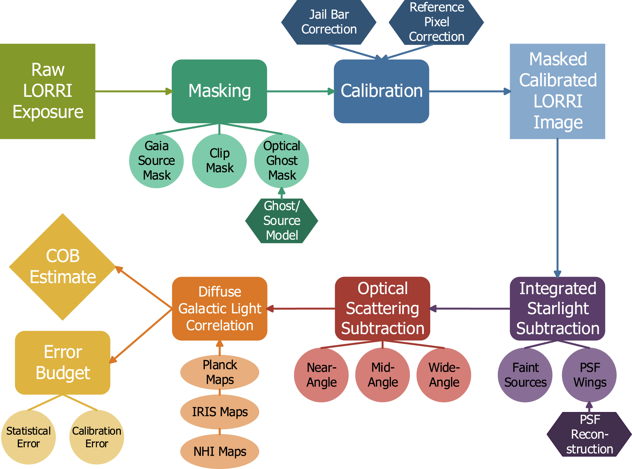
Figure 22. Comparison of ν bλ with previous measurements. The pink star gives our estimate of ν bλ combined from the estimates made using the IRIS, IRIS/SFD, and Planck templates. Again, the horizontal bar gives LORRI's wavelength range. The error bars indicate the combined δ ν bλ . Previous studies include Onishi et al. (2018), Sano et al. (2015, 2016a), Arai et al. (2015), Matsuoka et al. (2012), Ienaka et al. (2013), Guhathakurta & Tyson (1989), Laureijs et al. (1987), Paley et al. (1991), Zagury et al. (1999), Witt et al. (2008), Kawara et al. (2017), Tsumura et al. (2013b), Brandt & Draine (2012).
Download figure:
Standard image High-resolution image
Due to our lack of knowledge of the input fiducial values, we do not formally carry the uncertainties from these effects on our quoted COB result, but we estimate that a reduction of as much as several nW m−2 sr−1 in the final COB brightness could result from combinations of these kinds of effects. Further, the isotropic offsets in the DGL brightness are difficult to constrain at the level of the CIB brightness, and will impose uncertainties at the nW m−2 sr−1 level in the COB at our current level of understanding of the CIB absolute intensity. We conclude that the DGL scaling likely dominates the COB measurement error budget, and that more work should be done to constrain the bλ relation at optical wavelengths in the future.
Measurements of the relation between optical brightness and NHI column density are uncommon in the literature (Leinert et al. 1998), but Toller (1981) finds a relationship of the following:

with an unassessed uncertainty from Pioneer 10 data (Leinert et al. 1998). To provide a point of comparison, we recompute the scaling excluding the effect of d(b) and find a value of 1.92 ± 0.52 nW m−2 sr−1/1020 atoms cm−2. The excellent match between the COB brightness inferred from the NHI and thermal IR templates is strong evidence that the COB is unexpectedly high compared with models and galaxy counts.
In addition to astrophysical explanations, it is possible some things about the LORRI instrument and detector are causing a systematic misestimate of the COB. Although both we and others have attempted to bound or rule out these effects, in some cases, the data are not sufficient in themselves to fully assess the possible systematic uncertainty. One such effect is dark current. It is well known that CCDs exposed to cosmic rays will exhibit increased dark current over time (Janesick et al. 1987). Although the LORRI reference pixels do not seem to have changed their characteristics over the course of the mission (Symons 2022), it could be that the radiation damage has differentially impacted the dark current in the light and reference pixels at a level that is difficult to observe. However, Lauer et al. (2021) performed a thorough test of LORRI's dark current and detected no significant change. A possibly related issue is the observed relationship between the reference pixels and the light pixels discussed in Section 3.3. Although we derive and correct for an empirical relationship between these quantities, it is puzzling that there is a systematic offset between them in the first place. Applying the nominal surface brightness gain to the offset between the pixel populations, we find this offset corresponds to 16.9 nW m−2 sr−1, which in amplitude could explain the discrepancy between the measured COB and the expected IGL. Finally, the relaxation time of the detector following power-on appears to have a time constant of about 100 s, but we are not able to track the behavior over very long timescales. It is possible that the detector response following the power-on has multiple time constants that would only become apparent when the instrument is powered for long timescales that would source unaccounted systematics in this measurement. The data that are available in the archive are not sufficient to constrain these kinds of effects beyond what we have done. Although we have no evidence that any of the corrections we apply are incorrect, these issues do highlight the difficulty associated with systematic instrumental effects as well as the need for a dark shutter to help reliably track the subtle changes in the instrument over years.
Perhaps the most straightforward explanation for an excess of diffuse emission is that our IGL expectation is incorrect, and the galaxy counts have a deficit (Conselice et al. 2016). If this is true, upcoming JWST results will likely provide at least a partial resolution due to the telescope's unprecedented ability to detect faint, previously unseen galaxy populations (Gardner et al. 2006). Also of concern is if known galaxy populations have significant extended diffuse emission that has not been properly measured. IHL has also been extremely difficult to measure because it is both very faint and intrinsically diffuse. However, IHL from low-redshift sources has the potential to explain excess emission (Cooray et al. 2012; Zemcov et al. 2014; Cheng et al. 2021). Another proposed source of diffuse emission is faint compact objects (FCO), which could take the form of mini-quasars. These low-redshift objects are proposed to source a large amount of baryonic mass despite being difficult to detect (Matsumoto & Tsumura 2019). JWST should be able to detect FCOs directly if they are the correct explanation. High-redshift primordial black holes are another proposed source. Also referred to as direct collapse black holes, these objects may also provide an explanation for high-mass, high-redshift quasars (Cappelluti et al. 2013). Even though the current γ-ray measurements tend to align more closely with the expected IGL, a dense population of dark matter particles could have the potential to prevent pair-production as γ-rays travel long distances, which could result in an underestimate of γ-ray attenuation. This could result in γ-ray measurements more aligned with photometric EBL measurements than those from the IGL expectation (Biteau & Meyer 2022). An alternative explanation for the LORRI COB excess is an origin related to particle decays, especially axion-like particles (ALPs) with a mass in the range of 0.5–10 eV (Gong et al. 2016; Kohri & Kodama 2017; Bernal et al. 2022b). In addition to the mean intensity, such decays are expected to leave a large anisotropy signal in the COB and can be measured with anisotropy power spectra (e.g., CIBER; Zemcov et al. 2014; Hubble Space Telescope, hereafter HST; Mitchell-Wynne et al. 2015). A recent analysis of COB intensity and fluctuations power spectra finds evidence for ALP decays of ∼9.1 eV particles at the 2σ level (Bernal et al. 2022a). It is expected that the shorter wavelength optical and UV COB and anisotropy measurements can further constrain dark matter decays as a source of the intensity excess and will likely be targets for upcoming suborbital and space-based measurements using the small satellite architecture. Any of these proposed sources or some combination of all of them could together make up the observed excess.
Improved targeted measurements from more capable instruments will be necessary to resolve the current discrepancies between IGL and the photometrically determined COB. As of this writing, JWST has recently returned its first data, including a deep field observation that will likely revolutionize our understanding of galaxies in the universe (Gardner et al. 2006; Rigby et al. 2022). Upcoming missions such as SPHEREx (Crill et al. 2020), the first NIR all-sky spectral survey, and Euclid (Amendola et al. 2013), which will also measure galaxy redshifts, will provide unique opportunities for next-generation measurements of the EBL. However, these missions will still be located at 1 au and will suffer from the same foregrounds that have dogged COB measurements for decades. Even if ZL can be handled, both this COB measurement and previous measurements are critically dependent on the characterization and subtraction of the DGL, and undersubtraction (or oversubtraction) of DGL has an outsized impact on the scientific interpretation. Further study of the scaling between optical and FIR emission along with the scaling's dependence on sky position is necessary to resolve these disparate measurements. A dedicated small probe to the outer solar system, or a piggy-back instrument on a similar planetary or heliophysics mission, would be able to provide the best possible measurement (Cooray et al. 2009; Zemcov et al. 2018). One particularly intriguing mission concept is the Interstellar Probe (McNutt et al. 2019). The proposed 50 yr mission into interstellar space would provide an unparalleled opportunity to shed light on the EBL in the darkness between stars.
The work of T.S., M.Z., A.C., and A.R.P. was supported by the New Frontiers Data Analysis Program (NFDAP) under NASA grant 80NSSC18K1557. We would like to thank the LORRI team for advice, and the PDS archive team for help with both queries about the served LORRI data and assistance ingesting our final data products. The authors thank E. R. Imata for his assistance in archiving study results to the NASA Planetary Data System. Thanks to undergraduate research assistants S. Venuto, S. Thayer, A. Dignan, D. Houlihan, and A. Bush for their work on this project and V. Gorjian for comments that helped improve this work. This work has made use of data from the European Space Agency (ESA) mission Gaia, 6 processed by the Gaia Data Processing and Analysis Consortium (DPAC 7 . Funding for the DPAC has been provided by national institutions, in particular the institutions participating in the Gaia Multilateral Agreement. EBHIS is based on observations with the 100 m telescope of the Max-Planck-Institut für Radioastronomie (MPIfR) at Effelsberg. The Parkes Radio Telescope is part of the Australia Telescope, which is funded by the Commonwealth of Australia for operation as a National Facility managed by CSIRO.
Software: Astrobase (Bhatti et al. 2021), Astropy (Astropy Collaboration et al. 2013, 2018), gdpyc (Ruiz 2018), Matplotlib (Hunter 2007), NumPy (Van Der Walt et al. 2011), pandas (pandas development team 2020), and SciPy (Virtanen et al. 2020).
Footnotes
- 6
- 7