


Abstract
We present precise measurements of radial (RV) and projected rotational ( ) velocities of a sample of 258 M6 to L2 dwarfs with multiepoch, high-resolution (λ/Δλ = 22,500), near-infrared (1.514–1.696 μm) spectroscopic observations reported in the Apache Point Observatory Galactic Evolution Experiment Data Release 17. The spectra were modeled using a Markov Chain Monte Carlo forward-modeling method, which achieved median precisions of σRV = 0.4 km s−1 and
  = 1.1 km s−1. One-half of our sample (138 sources) are previously known members of nearby young clusters and moving groups, and we identified three new kinematic members of the Argus or Carina Near moving groups, 2MASS J05402570+2448090, 2MASS J14093200+4138080, and 2MASS J21272531+5553150. Excluding these sources, we find that the majority of our sample have kinematics consistent with the Galactic thin disk, and 11 sources are associated with the intermediate thin/thick disk. The field sample has a velocity dispersion of 38.2 ± 0.3 km s−1, equivalent to an age of 3.30 ± 0.19 Gyr based on empirical age–velocity dispersion relations, and a median
  of 17 km s−1. For 172 sources with multiepoch observations, we identified 37 as having significant RV variations, and determined preliminary orbit parameters for 26 sources with four or more epochs, nine of which are short-period binary candidates. For 40 sources with photometric variability periods from the literature less than 5 days and
  > 20 km s−1, we find a decline in projected radii (
 ) with age congruent with evolutionary models. Finally, we also present multiepoch RV and
  measurements for additional 444 candidate ultracool dwarfs.
Export citation and abstract BibTeX RIS

Original content from this work may be used under the terms of the Creative Commons Attribution 4.0 licence. Any further distribution of this work must maintain attribution to the author(s) and the title of the work, journal citation and DOI.
1. Introduction
Ultracool dwarfs (UCDs) are stellar and substellar objects with effective temperatures below 3000 K, masses below 0.1 M⊙, and spectral types spanning the late-M, L, T, and Y dwarf classes (Kirkpatrick 2005; Burgasser et al. 2006; Cushing et al. 2011). Over the past two decades, tens of thousands of UCDs have been discovered through large sky surveys such as the Two Micron All Sky Survey (2MASS; Skrutskie et al. 2006), the Sloan Digital Sky Survey (SDSS; York et al. 2000), the Wide-field Infrared Survey Explorer (Cutri et al. 2012), and Gaia (Gaia Collaboration et al. 2018, 2021a). Given such a large sample of UCDs, statistically studies of their physical properties become possible, particularly through the use of high-resolution spectroscopy.
High-resolution spectroscopy provides several unique opportunities for characterizing the physical properties of stars. These data provide precise radial velocities (RVs), which combined with proper motions and distances yield 3D kinematics that can be used to determine membership in Galactic populations (thin/thick disk, halo; Bensby et al. 2003) and young clusters and moving groups (Gagné et al. 2018). The dispersion of spatial velocities can also be used to statistically infer population ages (Wielen 1977; Aumer & Binney 2009). Multiepoch precise RVs enable the identification of single-line or double-line low-mass binaries (e.g., Blake et al. 2010; Burgasser et al. 2016; Triaud et al. 2020; Hsu et al. 2023). Projected rotational velocities trace angular momentum evolution as a function of age and magnetic activity (Zapatero Osorio et al. 2006; Herbst et al. 2007; Irwin et al. 2011; Bouvier et al. 2014) and enable assessment of spin–orbit alignment in binary and exoplanet systems (the Rossiter–McLaughlin effect; McLaughlin 1924; Rossiter 1924; Triaud et al. 2010). High-resolution spectroscopy can also be used to measure elemental abundances, including rare species and isotopes (e.g., 13CO; Tsuji 2016; Souto et al. 2017; Crossfield et al. 2019), and detailed line modeling can be used to measure magnetic fields through Zeeman splitting, wavelength-dependent limb darkening, and map surface structure through Doppler imaging (e.g., Shulyak et al. 2010; Crossfield 2014).
Despite these opportunities, the current sample of reported high-resolution spectroscopy for UCDs is limited to a few hundred systems due to their intrinsic faintness and red/infrared spectral energy distributions (Hsu et al. 2021a). For comparison, the Apache Point Observatory Galactic Evolution Experiment (APOGEE; Majewski et al. 2017; Wilson et al. 2019), part of the SDSS (Blanton et al. 2017), provides high-resolution (λ/Δλ ∼ 22,500) near-infrared spectra (1.514–1.696 μm) of more than 730,000 stars (Abdurro'uf et al. 2022). The single-epoch spectra of APOGEE have provided the chemical abundances for planet hosts (Souto et al. 2017, 2018, 2020; Wilson et al. 2018), Galactic chemical populations (Cunha et al. 2015; Hayden et al. 2015; Bovy et al. 2016; Donor et al. 2020), and cluster kinematics (Ness et al. 2016; Da Rio et al. 2017). The acquisition of multiepoch spectra has enabled discovery of thousands of binary systems, including ∼4000 single-lined spectroscopic binary companions to giants (Price-Whelan et al. 2018) and >7000 double-lined spectroscopic binaries (SB2) among main-sequence stars (Skinner et al. 2018; Kounkel et al. 2021). However, APOGEE does not provide robust RVs and  values for UCDs, as both the APOGEE Stellar Parameter and Chemical Abundances Pipeline (ASPCAP; García Pérez et al. 2016) and the more recent RV pipeline Doppler (Nidever 2021) have difficulties fitting molecule-rich UCD spectra below Teff = 3500 K.
Attempts have been made to model APOGEE spectra through other means. Metallicities and abundances of early to mid-M dwarfs (M0–M5) have been extensively explored in Schmidt et al. (2016), Souto et al. (2017, 2018, 2020, 2021, 2022), Rajpurohit et al. (2018), and Wanderley et al. (2023). APGOEE UCDs were relatively less explored in the literature. For example, Birky et al. (2020) measured the Teff values, metallicities, and spectral types of 5875 M dwarfs across M0 to M9 using a data-driven approach. Skinner et al. (2018) identified 44 M dwarf double-lined spectral binaries among a sample of 1350 M dwarfs.
17
Deshpande et al. (2013) reported RV and  measurements for 253 M dwarfs with APOGEE data using a forward-modeling approach. However, the sample is dominated by early to mid-M dwarfs, with only 27 sources falling in the UCD regime.
18
As discussed below, there are in fact hundreds of UCDs with APOGEE data. Additionally, the RVs reported by Deshpande et al. (2013) were determined by χ2 minimization using BT-Settl models (Allard et al. 1997). As shown in this paper, these older atmosphere models are unable to provide robust RVs and
measurements for 253 M dwarfs with APOGEE data using a forward-modeling approach. However, the sample is dominated by early to mid-M dwarfs, with only 27 sources falling in the UCD regime.
18
As discussed below, there are in fact hundreds of UCDs with APOGEE data. Additionally, the RVs reported by Deshpande et al. (2013) were determined by χ2 minimization using BT-Settl models (Allard et al. 1997). As shown in this paper, these older atmosphere models are unable to provide robust RVs and  values in the UCD regime due to missing FeH opacities. Gilhool et al. (2018) measured
  for 714 M dwarfs, with 17 M6–M8 in their sample. More recently, Sarmento et al. (2021) analyzed 313 M dwarfs to measure RV and
  using high signal-to-noise ratio (S/N > 200) spectra (but included 37 lower S/N benchmark sources to calibrate and explore their measurement limits). Due to their selection criteria for high S/N spectra, only one UCD, M8e 2MASS J05392474+4038437, was selected in their sample. The availability of several more UCD APOGEE spectra in Data Release 17 (DR17; Abdurro'uf et al. 2022) and improvements in stellar modeling motivate a reevaluation of these data, with the aim of building a larger and more precise sample of accurate RV and
  for UCDs.
In this article, we present multiepoch measurements of precise radial and projected rotational velocities for 258 spectroscopically classified and 444 candidate UCDs in the APOGEE sample, using a Markov Chain Monte Carlo (MCMC) forward-modeling method. This approach has been shown to provide precise and robust RV and  measurements for high-resolution near-infrared spectra of late-M, L, and T dwarfs (Blake et al. 2010; Burgasser et al. 2016; Hsu et al. 2021a), and here we apply the method to APOGEE observations of UCDs. In Section 2, we define our sample, including low-resolution optical spectra of 12 sources without prior classifications in the literature. In Section 3, we describe our forward-modeling approach in detail. In Section 4, we discuss our RV and
  measurements, and inferred effective temperatures and surface gravities, based on our fits. In Section 5, we combine our RV measurements with Gaia astrometry to determine 3D spatial motions, and use these to characterize Galactic populations and orbits, cluster memberships, and kinematic ages for the sample. We identify potential spectroscopic binary candidates among sources with multiepoch observations, and make preliminary orbit fits for 26 sources with four or more epochs of data. We also examine rotational velocity statistics, including trends with spectral type and distributions of projected radii and rotation axis inclinations for sources with published photometric variability periods. We summarize our key results in Section 6.
2. Sample and Observations
2.1. Sample Construction
Our UCD sample was curated from APOGEE DR17 (Abdurro'uf et al. 2022) of SDSS-IV (Blanton et al. 2017) based on observations obtained with the 2.5 m Sloan Foundation Telescope at the Apache Point Observatory (Gunn et al. 2006) and the 2.5 m du Pont Telescope at the Las Campanas Observatory (Bowen & Vaughan 1973). The majority of our targets were proposed in two SDSS Ancillary Science Programs, SDSS-III Project 176 (PIs: Suvrath Mahadevan and Cullen Blake; "A Radial Velocity Survey of Bright M Dwarfs with APOGEE: Companions,  , Fe/H") and SDSS-IV Project 288 (PI: Adam Burgasser; "APOGEE-2 and eBOSS Observations of the Lowest-Mass Stars and Brown Dwarfs in the Solar Neighborhood").
19
These programs are well aligned with one of the main stellar science goals of the APOGEE survey, which is the identification of close binary systems and substellar companions through RV variables (Blanton et al. 2017). We drew all of our sources from the DR17 allStar catalog,
20
and constructed two UCD samples for our analysis dubbed the "gold" and "full" samples. The analysis in this paper focuses on the gold sample. We present the construction and measurements of the full sample in the Appendix A.
, Fe/H") and SDSS-IV Project 288 (PI: Adam Burgasser; "APOGEE-2 and eBOSS Observations of the Lowest-Mass Stars and Brown Dwarfs in the Solar Neighborhood").
19
These programs are well aligned with one of the main stellar science goals of the APOGEE survey, which is the identification of close binary systems and substellar companions through RV variables (Blanton et al. 2017). We drew all of our sources from the DR17 allStar catalog,
20
and constructed two UCD samples for our analysis dubbed the "gold" and "full" samples. The analysis in this paper focuses on the gold sample. We present the construction and measurements of the full sample in the Appendix A.
Our "gold" sample was based on sources with classifications of M6 and later as reported in SIMBAD (Wenger et al. 2000), the Late-Type Extension to MoVeRS (Theissen et al. 2016, 2017), Reylé (2018), Best et al. (2021), or reported in this work. We use the most recent spectroscopic classification as our adopted value. Two sources were rejected from the sample based classifications earlier than M6 from additional follow-up spectroscopy discussed below. We validated the remaining sources by visually inspecting optical (SDSS) and near-infrared images (2MASS), and confirmed correct placement on color–magnitude and color–color diagrams combining 2MASS and Gaia EDR3 (Gaia Collaboration et al. 2021a) photometry and astrometry (Figure 1). We further imposed a limit on the median spectral S/N of the APOGEE data to be >10. After removal of spectral type earlier than M6 using our optical spectra (Section 2.2) and color-type relation from Kiman et al. (2019), these criteria resulted in a sample of 931 spectra of 258 sources summarized in Table 1, which is the gold sample.

Figure 1. Color–magnitude properties of the UCD APOGEE sample. The full sample is indicated by gray dots, the gold sample by dots color coded with spectral type. Blue stars highlight spectroscopic binary candidates. Top: MG vs. G − J. Bottom: G − J vs. J − K.
Download figure:
Standard image High-resolution imageTable 1. APOGEE DR17 Gold Sample
| APOGEE ID | R.A. | Decl. | Gaia eDR3 Source ID | SpT | SpT References | Nobs | 2MASS H | μα | μδ | μ References | π | π References |
|---|---|---|---|---|---|---|---|---|---|---|---|---|
| (deg) | (deg) | (mag) | (mas yr−1) | (mas yr−1) | (mas) | |||||||
| 2MASS J00034394+8606422 | 0.933088 | +86.111732 | 574059045248283008 | M6.0 | (93) | 10 | 11.738 ± 0.031 | 175.94 ± 0.04 | −25.83 ± 0.04 | (99) | 30.81 ± 0.03 | (99) |
| 2MASS J00312793+6139333 | 7.866401 | +61.659252 | 430215470915266560 | M7 | (79, 97) | 6 | 12.483 ± 0.028 | 369.52 ± 0.07 | 158.0 ± 0.07 | (99) | 27.86 ± 0.07 | (99) |
| 2MASS J00381273+3850323 | 9.553082 | +38.842308 | 368514898441866368 | M6 | (91) | 6 | 12.459 ± 0.033 | 163.84 ± 0.05 | 12.5 ± 0.05 | (99) | 17.21 ± 0.06 | (99) |
| 2MASS J00452143+1634446 | 11.339304 | +16.579082 | 2781513733917711616 | L2beta | (44) | 3 | 12.059 ± 0.035 | 359.07 ± 0.2 | −47.91 ± 0.14 | (99) | 65.41 ± 0.18 | (99) |
| 2MASS J00514593−1221458 | 12.941377 | −12.362734 | 2376328546438257536 | M6.1 | (93) | 2 | 11.89 ± 0.022 | −32.76 ± 0.06 | −38.85 ± 0.06 | (99) | 26.36 ± 0.04 | (99) |
| 2MASS J01154176+0059317 | 18.924037 | +0.992157 | 2535273088355573120 | M6 | (100) | 2 | 12.651 ± 0.027 | 163.82 ± 0.15 | 24.1 ± 0.13 | (99) | 15.77 ± 0.13 | (99) |
| 2MASS J01215816+0101007 | 20.492347 | +1.016877 | 2535133209860543616 | M6.5 | (100) | 2 | 12.429 ± 0.026 | 161.94 ± 0.16 | −78.8 ± 0.09 | (99) | 26.49 ± 0.12 | (99) |
| 2MASS J01243124−0027556 | 21.130173 | −0.465459 | 2533946665015570304 | M7 | (51) | 2 | 11.506 ± 0.029 | 66.72 ± 0.32 | −170.47 ± 0.18 | (99) | 29.17 ± 0.25 | (99) |
| 2MASS J01514363+0046188 | 27.931833 | +0.771889 | 2510880216734767232 | M7 | (87) | 3 | 12.431 ± 0.023 | 126.98 ± 0.12 | 30.41 ± 0.08 | (99) | 26.32 ± 0.1 | (99) |
| 2MASS J02163612−0544175 | 34.150527 | −5.73821 | 2487920936478100992 | M6.1 | (93) | 3 | 11.787 ± 0.029 | 23.79 ± 0.06 | −79.67 ± 0.05 | (99) | 30.91 ± 0.05 | (99) |
References: (1) Stephenson (1986); (2) Kirkpatrick et al. (1991); (3) Reid et al. (1995); (4) Rebull et al. (2000); (5) Ardila et al. (2000); (6) Gizis et al. (2000); (7) Jahreiß et al. (2001); (8) Martín et al. (2001); (9) McCaughrean et al. (2002); (10) Henry et al. (2002); (11) Hawley et al. (2002); (12) Preibisch et al. (2002); (13) Gizis (2002); (14) Briceño et al. (2002); (15) Monet et al. (2003); (16) Lépine et al. (2003); (17) Cruz et al. (2003); (18) Reid et al. (2003); (19) Luhman et al. (2003); (20) Martín et al. (2004); (21) Wilking et al. (2004); (22) Henry et al. (2004); (23) Luhman (2004); (24) Crifo et al. (2005); (25) Wilking et al. (2005); (26) Meeus & McCaughrean (2005); (27) Reid & Gizis (2005); (28) Guieu et al. (2006); (29) Slesnick et al. (2006a); (30) Slesnick et al. (2006b); (31) Luhman et al. (2006); (32) Law et al. (2006); (33) Menten et al. (2007); (34) Cruz et al. (2007);(35) Schmidt et al. (2007); (36) Reid et al. (2007); (37) Muench et al. (2007); (38) Kraus & Hillenbrand (2007); (39) Close et al. (2007); (40) Reid et al. (2008); (41) Peterson et al. (2008); (42) Slesnick et al. (2008); (43) Phan-Bao et al. (2008); (44) Cruz et al. (2009); (45) Currie & Kenyon (2009); (46) Monin et al. (2010); (47) Winston et al. (2010); (48) Konopacky et al. (2010); (49) Lodieu et al. (2011); (50) Faherty et al. (2011); (51) West et al. (2011); (52) Becker et al. (2011); (53) Sicilia-Aguilar et al. (2011); (54) Kirkpatrick et al. (2011); (55) Melnikov & Eislöffel (2012); (56) Deshpande et al. (2012); (57) Scholz et al. (2012); (58) Zacharias et al. (2012); (59) Hillenbrand et al. (2013); (60) Aller et al. (2013); (61) Newton et al. (2014); (62) Mann et al. (2014); (63) Esplin et al. (2014); (64) Dittmann et al. (2014); (65) Bardalez Gagliuffi et al. (2014); (66) Dawson et al. (2014); (67) Schmidt et al. (2014); (68) Cutri et al. (2021); (69) Alonso-Floriano et al. (2015); (70) Manara et al. (2015); (71) Gagné et al. (2015b); (72) West et al. (2015); (73) Gagné et al. (2015a); (74) Cook et al. (2016); (75) Luhman et al. (2017); (76) Theissen et al. (2017); (77) Esplin & Luhman (2017); (78) Dupuy & Liu (2017); (79) Reylé (2018); (80) Esplin et al. (2018); (81) Luhman et al. (2018); (82) Zhang et al. (2018); (83) Theissen (2018); (84) Bai et al. (2018); (85) Ahmed & Warren (2019); (86) Cazzoletti et al. (2019); (87) Kiman et al. (2019); (88) Lu et al. (2019); (89) Zhong et al. (2019); (90) Cabello et al. (2019); (91) Guo et al. (2019); (92) Luhman & Esplin (2020); (93) Birky et al. (2020); (94) Tian et al. (2020); (95) Allers & Liu (2020); (96) Sebastian et al. (2021); (97) Best et al. (2021); (98) Esplin & Luhman (2022); (99) Gaia Collaboration et al. (2021a); and (100) this work.
Only a portion of this table is shown here to demonstrate its form and content. A machine-readable version of the full table is available.
Download table as: Machine-readable (MRT)Typeset image
Figure 2 displays the observable properties of our gold and full samples. The distribution of targets across the sky is highly dependent on APOGEE's survey pointings. Notably, half of the gold sample includes known members of nearby young moving groups (the Upper Scorpius and Taurus young associations), targeted as part of the programs described in Zasowski et al. (2013, 2017), Beaton et al. (2021), and Santana et al. (2021). The spectral types for our gold sample range from M6 to L2, with 252 late-M dwarfs and six L dwarfs. For the full sample that is not in the gold sample, the Gaia G − GRP–spectral type relation of Kiman et al. (2019) indicates spectral types of M4 to L4, with 184 late-M dwarfs and 17 L dwarfs. The majority of our gold sample (80%) and full sample (90%) have distances larger than 30 pc, with the M6.5Ve G 51−15 (2MASS J08294949+2646348) being the closest source at a Gaia distance of 3.5810 ± 0.0008 pc. The apparent H-band magnitudes of our targets extend to 14.65, which is slightly fainter than the APOGEE magnitude limit of 13.8 for S/N = 100.

Figure 2. Distributions of observables for the APOGEE UCD sample. Gold sample sources are indicated by blue lines and symbols and full sample sources are indicated by black lines and symbols, Top left: sky distribution of our samples in Galactic coordinates. Known young sources in our gold sample are highlighted by red squares, and the major two clusters Upper Scorpius (USCO) and Taurus (TAU) are labeled in red text near the cluster locations. The Galactic latitudes at ±15° are shown in gray dashed lines. Top right: spectral type distributions for our samples, and gold sample spectral types drawn from the literature (see Table 1 for references) or observations presented here, and full sample spectral types estimated from the Kiman et al. (2019) Gaia G − GRP–spectral type relation. Dashed line histograms indicate the distributions of sources with four or more observation epochs. Bottom left: Gaia EDR3 parallax measurement distributions for our samples. Note that the maximum distance value is 400 pc. The single source within 10 pc (π > 100 mas) is the M6.5Ve G 51−15 (2MASS J08294949+2646348). Bottom right: apparent 2MASS H-band magnitude distributions for our samples. The S/N limit = 100 (H ∼ 13.8 mag) is labeled in the vertical black dashed line.
Download figure:
Standard image High-resolution imageThe majority of both samples (66% and 51%) have APOGEE spectral observations taken over multiple epochs, enabling more precise determinations of RVs and the possibility of measuring RV variations. We defined multiepoch subsamples in our gold and full samples as those with at least four observations satisfying S/N > 10, each separated by at least 0.85 day. A total of 71 sources in the gold sample and 115 sources in the full sample satisfy these criteria, and the RV variables among the subsample are discussed in Section 5.5.
Finally, we note that the requirement for a Gaia detection likely resulted in the rejection of true UCDs in the full sample due to sensitivity limitations (Theissen 2018), and APOGEE targeting was not intended to be uniform across the sky (Zasowski et al. 2013). Therefore, our APOGEE UCD sample is not expected to be magnitude or volume complete, but rather representative of the broader UCD population.
2.2. Additional Spectral Observations
The majority of sources in our full sample lack published spectroscopic classifications.
21
To bolster this sample, we obtained additional low-resolution optical spectra with the Kast Double Spectrograph (Miller & Stone 1994) on the Shane 3 m Telescope at the Lick Observatory over multiple nights between 2018 January 21 and 2022 March 11. We used the 600/7500 grating and 2'' slit to obtain 6000–9000 Å spectra at an average resolution of λ/Δλ ≈ 1800. Data acquisition included observations of flat-field and arc lamps for pixel response and wavelength calibration, nightly observations of a spectral flux standard from Hamuy et al. (1992, 1994) for relative flux calibration, and observations of a nearby G2 V or A0 V star at similar air mass for telluric absorption and continuum correction. All data were reduced using the kastredux package
22
using default settings. An example spectrum of the M9 dwarf 2MASS J21272531+5553150 (aka LSPM J2127+5553) is shown in Figure 3. Table 2 summarizes the observations and corresponding measurements. Spectral classifications were determined by the closest match to SDSS dwarf spectral templates from Bochanski et al. (2007b), Schmidt et al. (2014), and Kesseli et al. (2017), and indicate types ranging from M5 to M9. Metallicity index (ζ) measurements (Lépine et al. 2007) are uniformly greater than 0.9 and indicate near-solar metallicities for all sources. We detected Hα emission in all of the sources, and measured relative Hα emission luminosity ( ) from equivalent widths and the χ factor relations of Douglas et al. (2014) and Schmidt et al. (2014); these values range over −4.9 <
  < −3.8.

Figure 3. Normalized Shane/Kast spectrum of 2MASS J21272531+5553150 (black line) compared to the best-match M9 spectral template from Bochanski et al. (2007b, magenta line). The lower panel compares the difference between these spectra to the measurement uncertainty (gray band). The inset box highlights the region around Hα emission at 6563 Å and Li i absorption at 6708 Å.
Download figure:
Standard image High-resolution imageTable 2. Shane/Kast Observations of APOGEE Targets
| 2MASS Source ID | Obs. Date | Air Mass | Exp. Time | S/N a | SpT b | ζc |
 d
d
|
|---|---|---|---|---|---|---|---|
| (UT) | (s) | ||||||
| 2MASS J14554964+0321420 | 2021 May 15 | 1.21 | 2400 | 73 | M5.0 | 1.195 ± 0.004 | −4.81 ± 0.12 |
| 2MASS J15042797+0942464 | 2021 May 15 | 1.42 | 3000 | 47 | M5.0 | 1.093 ± 0.007 | −3.75 ± 0.08 |
| 2MASS J07552256+2755318 | 2021 Nov 27 | 1.02 | 3000 | 130 | M6.0 | 1.118 ± 0.002 | −4.01 ± 0.09 |
| 2MASS J11210854+2126274 | 2021 May 15 | 1.05 | 2400 | 97 | M6.0 | 1.048 ± 0.002 | −4.11 ± 0.09 |
| 2MASS J08080189+3157054 | 2021 Jan 17 | 1.11 | 3000 | 55 | M7.0 | 1.007 ± 0.003 | −4.22 ± 0.16 |
| 2MASS J12215013+4632447 | 2018 Jan 21 | 1.02 | 2400 | 156 | M7.0 | 1.008 ± 0.001 | −4.17 ± 0.16 |
| 2MASS J13342918+3303043 | 2020 Feb 5 | 1.02 | 3600 | 84 | M7.0 | 1.031 ± 0.002 | −4.91 ± 0.12 |
| 2MASS J16572919+2448509 | 2022 Mar 11 | 1.06 | 3000 | 113 | M7.0 | 0.919 ± 0.002 | −4.05 ± 0.13 |
| 2MASS J21381698+5257188 | 2020 Dec 14 | 1.22 | 3000 | 85 | M7.0 | 1.005 ± 0.002 | −4.17 ± 0.14 |
| 2MASS J12493960+5255340 | 2021 May 16 | 1.06 | 3000 | 16 | M9.0 | 1.506 ± 0.043 | −4.93 ± 0.14 |
| 2MASS J19544358+1801581 | 2020 Aug 14 | 1.07 | 3600 | 98 | M9.0 | 1.207 ± 0.003 | −4.70 ± 0.11 |
| 2MASS J21272531+5553150 | 2020 Aug 14 | 1.06 | 3600 | 96 | M9.0 | 1.080 ± 0.003 | −4.78 ± 0.10 |
Notes.
a Median S/N in the 7200–7400 Å region. b Closest match to the SDSS dwarf spectral templates defined in Bochanski et al. (2007b), Schmidt et al. (2014), and Kesseli et al. (2017). c Metallicity index defined in Lépine et al. (2007), where ζ > 0.875 indicates a dwarf (solar) metallicity classification. d Relative luminosity in Hα emission based on the measured Hα equivalent width and χ correction factors compiled by Douglas et al. (2014) and Schmidt et al. (2014).Download table as: ASCIITypeset image
3. APOGEE Spectral Analysis
3.1. Spectral Data
Spectra were drawn from the APOGEE single-epoch, individual visit spectra (apVisit) files (Abdurro'uf et al. 2022), covering chips a (1.657–1.696 μm), b (1.585–1.644 μm), and c (1.514–1.581 μm). APOGEE data reduction is described in detail in Nidever et al. (2015), Holtzman et al. (2018), Jönsson et al. (2020), and Abdurro'uf et al. (2022). Each apVisit spectrum underwent dark, flat-field, cosmic-ray, flux, sky, and telluric corrections, as well as wavelength calibrations. In particular, the wavelength solutions were derived from a combination of sky lines and ThArNe and UNe hollow-cathode lamps (Nidever et al. 2015). Bad pixels were masked out using the bit mask for each chip. 23 In order to simultaneously calibrate the wavelength solution imprinted in the spectra, the telluric absorption profile has been retained for each reduced apVisit spectrum (HDU7).
3.2. Forward Modeling
To infer the physical properties of our sources—effective temperature (Teff), surface gravity ( ), RV, and rotational velocity (
 )—we employed an MCMC forward-modeling technique that simultaneously models the telluric and stellar absorption present in each APOGEE apVisit spectrum. We used the Spectral Modeling Analysis and RV Tool (SMART; Hsu et al. 2021b), which follows methods previously described in Blake et al. (2010), Burgasser et al. (2016), Theissen et al. (2022), and Hsu et al. (2021a).
Each APOGEE spectrum is forward modeled using the following equation:

Here, D[p] is the data model as a function of pixel p; C[p] is a fifth-order polynomial representing a continuum correction; M[p] is the stellar solar-metallicity atmosphere model parameterized by Teff and  ; p*(λ) is a wavelength-to-pixel conversion function, initially provided by the APOGEE reduction pipeline with an additional constant offset parameter CΔλ
to adjust for chip-to-chip variations; RV* = RV + vbary is the RV of the source plus the barycentric motion of the Earth at the observed epoch; c is the speed of light; κD
is a Gaussian convolution kernel that applies a microturbulence velocity broadening νmicro, modeled as 2.478 – 0.325
; p*(λ) is a wavelength-to-pixel conversion function, initially provided by the APOGEE reduction pipeline with an additional constant offset parameter CΔλ
to adjust for chip-to-chip variations; RV* = RV + vbary is the RV of the source plus the barycentric motion of the Earth at the observed epoch; c is the speed of light; κD
is a Gaussian convolution kernel that applies a microturbulence velocity broadening νmicro, modeled as 2.478 – 0.325  km s−1 (Zamora et al. 2015); κR
is a rotational line broadening convolution kernel for projected rotational velocity
km s−1 (Zamora et al. 2015); κR
is a rotational line broadening convolution kernel for projected rotational velocity  , with linear limb-darkening coefficient
  = 0.6 (Gray 1992); T[p] is the telluric absorption model based on the model grid of Moehler et al. (2014) and parameterized by air mass and precipitable water vapor; κG
is a Gauss–Hermite convolution kernel used to account for the instrumental line-spread function (LSF), with width νinst obtained from the APOGEE pipeline (Nidever et al. 2015; Bovy 2016); and Cflux is a constant additive flux offset.
= 0.6 (Gray 1992); T[p] is the telluric absorption model based on the model grid of Moehler et al. (2014) and parameterized by air mass and precipitable water vapor; κG
is a Gauss–Hermite convolution kernel used to account for the instrumental line-spread function (LSF), with width νinst obtained from the APOGEE pipeline (Nidever et al. 2015; Bovy 2016); and Cflux is a constant additive flux offset.
The log-likelihood function of our model fit was defined as

where the statistic

compares the observed spectrum S[p] and uncertainty σ[p] to the scaled forward model D[p], with the scale factor α determined to minimize χ2. We include the constant scaling factor Cnoise to account for under estimation of observational noise, as well as systematic errors such as missing line features.
Cool dwarfs have abundant molecular absorption lines in their infrared spectra, and hence careful consideration must be made for the choice of stellar model. We explored synthetic model grids from Baraffe et al. (2015, BT-Settl CIFIST models), Husser et al. (2013, ACES models), Gustafsson et al. (2008, MARCS models), and Marley et al. (2018, Sonora models). For the lowest-temperature dwarfs (L dwarfs), we found that the Sonora models outperform other model sets, particular redward of 1.58 μm where FeH absorption is an important source of opacity (Cushing et al. 2003; Souto et al. 2017), although there are still some missing features in chip c.
For each source and model set, we fit all three chips simultaneously, with the nuisance parameters Cflux, CΔλ , and continuum parameters modeled separately for each chip. The 18 continuum parameters, LSF broadening, νmicro, and vbary were fit and applied at the end of the MCMC loop, leaving 13 parameters to be fit by the forward-modeling routine, summarized in Table 3. Priors for these parameters were assumed to be uniformly distributed between bounds based on expected values for late-M and L dwarfs or model parameter limits. We used the emcee code (Foreman-Mackey et al. 2013) to run the MCMC with kernel density estimator (KDE) 24 moves, which allows efficient convergence of best-fit parameters. We deployed 100 chains of 1000 steps each, with the first 800 steps removed for burn-in. At step 600, we used a 3σ-clipping mask of data minus model residuals to remove outlying flux values, which were mostly unmasked bad pixels and discrepant opacities. Chains were visually inspected to ensure convergence, and the typical integrated autocorrelation range was ∼17 steps. We report best-fit parameters as the median of the tails of the chains, with uncertainties derived from the 16% to 84% quantile range.
Table 3. Forward-modeling Parameters
| Description | Symbol (Unit) | Priors a | Bounds |
|---|---|---|---|
| Temperature | Teff (K) | (1800, 4000) b | (1200, 7000) b |
| ⋯ | ⋯ | (1500, 2400) c | (200, 2400) c |
| Surface Gravity |
 (cm s−2) (cm s−2) | (3.5, 5.5) | (3.5, 5.5) |
| Rotational Velocity |
 (km s−1) (km s−1) | (0, 50) | (0, 100) |
| Radial Velocity | RV (km s−1) | (−100, +100) | (−200, +200) |
| Flux Offset d | Cflux | (−0.01, +0.01) | (−104, +104) |
| Wave Offset d | CΔλ (Å) | (−0.1, +0.1) | (−0.5, +0.5) |
| Air Mass | AM | (1.0, 3.0) | (1.0, 3.0) |
| Water Vapor | PWV (mm) | (0.5, 20.0) | (0.5, 20.0) |
| Noise Factor | Cnoise | (1.0, 5.0) | (1.0, 10.0) |
Notes.
a All priors assume a uniform distribution over the range specified. b Teff range for the BT-Settl models. c Teff range for the Sonora models. d The three APOGEE chips were fit individually.Download table as: ASCIITypeset image
We note that one-half of our sample are young sources, and hence magnetic emission as traced by the Bracket hydrogen emission series (e.g., Br 16 → 4, λ = 1.556 μm; Br 15 → 4, λ = 1.571 μm; Br 13 → 4, λ = 1.611 μm; Br 11 → 4, λ = 1.681 μm; see Sullivan et al. 2019) could be present in some sources. None of the models used include hydrogen emission; however, any such emission was much weaker compared to other absorption lines, as verified by visual inspection of each best-fit spectrum. 25
To assess the quality of these fits, Figures 4–6 show the best-fit models using Sonora and BT-Settl models for the L2β 2MASS J00452143+1634446, the M9 2MASS J08440350+0434356, and the M7 + M9.5 binary 2MASS J04214955+1929086, respectively. The Sonora models clearly outperform the other models based on the residuals and χ2 fit values, even though the best-fit Teff reaches the Teff limits of the Sonora model grid. The best-fit models of the BT-Settl, ACES, and MARCS models give similar results, with significant residuals redward of 1.58 μm driving up the χ2 values. The Sonora models incorporate the Hargreaves et al. (2010) FeH E4Π − A4Π transitions (1.58263 μm, 1.59188 μm, and 1.62457 μm bandheads covering from 1.58 to 1.75 μm; Wallace & Hinkle 2001; Cushing et al. 2005), and we thus attribute residuals in the other models to outdated FeH opacities. The other models also yield lower  and higher
  values than the Sonora models, which we interpret as compensation for these missing opacities; a similar effect for methane from Yurchenko & Tennyson (2014) has been noted in J-band spectra of T dwarfs (Hsu et al. 2021a).

Figure 4. Spectrum and best-fit forward models for the APOGEE spectrum of the L2β 2MASS J00452143+1634446 observed on JD 2456587.736. The APOGEE data are labeled in black, and the best-fit forward models with Sonora and BT-Settl models are labeled in blue and magenta, respectively. The noise and residual (data − model) are depicted in gray shaded regions and colored lines corresponding to the models, respectively. Parameter values and their uncertainties are listed at the top of the panel.
Download figure:
Standard image High-resolution image
Figure 5. Same as Figure 4 for the APOGEE spectrum of the M9 2MASS J08440350+0434356 observed on JD 2458198.659.
Download figure:
Standard image High-resolution image
Figure 6. Same as Figure 4 for the APOGEE spectrum of the M7 + M9.5 2MASS J04214955+1929086 observed on JD 2458820.725.
Download figure:
Standard image High-resolution imageFor warmer sources (late-M dwarfs) the BT-Settl models provided superior fits to the Sonora and other models, although the telluric absorption strengths are higher for these model fits, again suggesting compensation for missing opacity. Based on these initial fits, we focused our analysis on these two model sets, with an "optimal model" transition, as verified by visual inspection of each fit, around 2700 K ≲ Teff ≲ 3000 K. At and below these transition temperatures, the Sonora models yield better fits even at its Teff = 2400 K parameter limit.
4. Results
In this section, we review our RV,  , Teff, and
  measurements, all of which are compiled in Table 4.
26
measurements, all of which are compiled in Table 4.
26
Table 4. Spectral Model Fit Parameters
| APOGEE ID | Plate | Loc. ID | Fiber ID | JD | Bary. a | S/N | RV b , c | 〈RV〉 b , c , d |
 b
b
|
 b
,
d
,
e
b
,
d
,
e
| Teff f | 〈Teff〉 d , f |
 f
f
|
 d
,
f
d
,
f
| Mdl g |
|---|---|---|---|---|---|---|---|---|---|---|---|---|---|---|---|
| (days) | (km s−1) | (km s−1) | (km s−1) | (km s−1) | (km s−1) | (K) | (K) | (cm s−2) | (cm s−2) | ||||||
| 2MASS J00034394+8606422 | 5221 | 4217 | 275 | 2455815.921 | 11.92 | 33 |

|

|

|

|

|

|

|

| S |
| ⋯ | 5221 | 4217 | 227 | 2455822.934 | 11.89 | 18 |

| ⋯ |

| ⋯ |

| ⋯ |

| ⋯ | S |
| ⋯ | 5221 | 4217 | 275 | 2455841.765 | 10.97 | 32 |

| ⋯ |

| ⋯ |

| ⋯ |

| ⋯ | S |
| ⋯ | 5221 | 4217 | 275 | 2455866.685 | 7.98 | 42 |

| ⋯ |

| ⋯ |

| ⋯ |

| ⋯ | S |
| ⋯ | 5221 | 4217 | 227 | 2455876.687 | 6.30 | 39 |

| ⋯ |

| ⋯ |

| ⋯ |

| ⋯ | S |
| ⋯ | 5221 | 4217 | 224 | 2456653.557 | −3.17 | 42 |

| ⋯ |

| ⋯ |

| ⋯ |

| ⋯ | S |
| ⋯ | 5221 | 4217 | 224 | 2456654.555 | −3.37 | 40 |

| ⋯ |

| ⋯ |

| ⋯ |

| ⋯ | S |
| ⋯ | 5221 | 4217 | 224 | 2456655.555 | −3.58 | 33 |

| ⋯ |

| ⋯ |

| ⋯ |

| ⋯ | S |
| ⋯ | 5221 | 4217 | 224 | 2456656.551 | −3.78 | 44 |

| ⋯ |

| ⋯ |

| ⋯ |

| ⋯ | S |
| ⋯ | 6104 | 4217 | 224 | 2456902.680 | 11.76 | 51 |

| ⋯ |

| ⋯ |

| ⋯ |

| ⋯ | S |
| 2MASS J00312793+6139333 | 6228 | 4243 | 131 | 2456171.848 | 16.15 | 29 |

|

|

| <10 |

|

|

|

| S |
| ⋯ | 6229 | 4243 | 134 | 2456172.852 | 15.99 | 28 |

| ⋯ |

| ⋯ |

| ⋯ |

| ⋯ | S |
| ⋯ | 6228 | 4243 | 122 | 2456177.838 | 15.18 | 32 |

| ⋯ |

| ⋯ |

| ⋯ |

| ⋯ | S |
| ⋯ | 6228 | 4243 | 125 | 2456202.709 | 9.62 | 28 |

| ⋯ |

| ⋯ |

| ⋯ |

| ⋯ | S |
| ⋯ | 6229 | 4243 | 137 | 2456203.752 | 9.28 | 34 |

| ⋯ |

| ⋯ |

| ⋯ |

| ⋯ | S |
| ⋯ | 6229 | 4243 | 137 | 2456223.734 | 3.27 | 27 |

| ⋯ |

| ⋯ |

| ⋯ |

| ⋯ | S |
Notes. Measurements from individual spectra over individual or multiple epochs are combined using inverse uncertainty weighting (weight =  ); upper and lower uncertainties are also combined using inverse uncertainty-squared weighting. In cases where individual spectra have S/N < 10, spectral data are combined first, then modeled.
 measurements, respectively. See Sections 4.1 and 4.2 for details.
c
We did not apply the effective temperature dependent correction to RV from Kounkel et al. (2019) for 2MASS J04201611+2821325, 2MASS J04262939+2624137, 2MASS J04294568+2630468, 2MASS J04330945+2246487, and 2MASS J04363893+2258119. See Section 4.1 for details.
d
Weighted average over all epochs.
e
Averaged
measurements, respectively. See Sections 4.1 and 4.2 for details.
c
We did not apply the effective temperature dependent correction to RV from Kounkel et al. (2019) for 2MASS J04201611+2821325, 2MASS J04262939+2624137, 2MASS J04294568+2630468, 2MASS J04330945+2246487, and 2MASS J04363893+2258119. See Section 4.1 for details.
d
Weighted average over all epochs.
e
Averaged  < 10 km s−1 is below our
  detection limit; see Section 4.2 for details.
f
Readers should not take our Teff and
detection limit; see Section 4.2 for details.
f
Readers should not take our Teff and  measurements as accurate. We report these values only for the reproducibility of our work. See Section 4.4 for details.
g
Models used: S = Sonora 2018 (Marley et al. 2018) and B = BT-Settl (Baraffe et al. 2015).
measurements as accurate. We report these values only for the reproducibility of our work. See Section 4.4 for details.
g
Models used: S = Sonora 2018 (Marley et al. 2018) and B = BT-Settl (Baraffe et al. 2015).
Only a portion of this table is shown here to demonstrate its form and content. A machine-readable version of the full table is available.
Download table as: Machine-readable (MRT)Typeset image
4.1. Radial Velocities
Our RV measurements span the range −76.08 to +66.68 km s−1 with a median value of −0.78 km s−1 and a median measurement uncertainty of 0.32 km s−1. To assess sources of systematic uncertainty, we evaluated the scatter in measurements inferred from 13 epochs of observations of the M2 2MASS J16495034+4745402, one of the RV standards in the Deshpande et al. (2013) APOGEE sample. We compared fits based on MARCS, BT-Settl, and ACES models, which had internal per-epoch scatter of 0.18 km s−1, 0.19 km s−1, and 0.16 km s−1, respectively, and an overall scatter between models of 0.18 km s−1. We therefore conservatively assume an overall systematic RV uncertainty of 0.19 km s−1, which has been added in quadrature to the reported RV measurements for all sources, resulting in a final median RV precision of 0.37 km s−1.
We explored whether this precision could be improved by modeling restricted wavelength regions where strong telluric absorption can be used to improve the wavelength calibration. This experiment was motivated by higher fitting scatter in regions that had by slight mismatches between the observed and modeled spectra, possibly due to offsets in the wavelength calibrations derived from arc lamp lines. We fit regions of strong telluric absorption at 16560–16700 Å on chip a, 15980–16160 Å on chip b, and 15100–15500 Å and 15500–16800 Å on chip c (see Figure 4), and included an additional pixel-to-wavelength zero-point offset term in our model. The resulting variance in RV measurements between these regions, 0.23–0.56 km s−1, was worse than fitting all three chips simultaneously, likely due to the lack of strong stellar lines. We conjecture that slight improvements in the APOGEE pipeline wavelength calibration could be realized by combining arc lines, sky emission lines, and telluric absorption lines to compute the overall wavelength calibration.
We quantified the validity of our RV measurements by comparing our measured RVs with those reported in the literature, summarized in Table 5. Excluding published RVs from APOGEE DR16 (Jönsson et al. 2020), a total of 67 sources in our sample have reported RVs in the literature with uncertainties. Figure 7 compares these values. The vast majority (84%) have consistent RVs to within 3σ deviation, while 11 sources are significant outliers.
- 1.Two of these outliers, 2MASS J08294949+2646348 (ΔRV = 5.5 km s−1), 2MASS J16311879+4051516 (ΔRV = 4.4 km s−1), are based on measurements made with lower-resolution data (λ/Δλ ≈ 2000) reported in Terrien et al. (2015b), and may reflect underestimated uncertainties.
- 2.Five other outliers, 2MASS J04201611+2821325, 2MASS J04262939+2624137, 2MASS J04294568+2630468, 2MASS J04330945+2246487, and 2MASS J04363893+2258119 are all members of the Taurus Complex star-forming region and have prior APOGEE measurements reported by Kounkel et al. (2019) that are 2–3 km s−1 lower than our measurements. Cottaar et al. (2014), Cook et al. (2014), and Kounkel et al. (2019) all report a systematic redshift in RV measurements among the lowest-temperature sources in their cluster samples (Teff ≤ 3400 K), and the last study proposes a systematic correction of ΔRV = 12.84 – 0.0038 × Teff. Accounting for this offset brings our measurements fully in line with RVs reported in Kounkel et al. (2019), but we did not report these corrected values in this work.
- 3.Another young source, the M6 2MASS J16093019−2059536, a reported member of the Upper Scorpius Association (Slesnick et al. 2006a), also has a significantly different RV from our measurements (RV = −1.3 ± 0.6 km s−1) compared to that reported in Dahm et al. (2012, RV = −5.1 ± 0.6 km s−1). The latter is based on optical high-resolution spectra and cross correlation with the M8 standard VB 10. On the other hand, our measurement is fully consistent with that reported in Jönsson et al. (2020, −0.98 ± 0.09 km s−1), using the cross-correlation method with DR16 APOGEE spectra. The variance between these measurements could again be due to the RV offset found among young low-temperature sources, or variability induced by a binary (only one epoch of APOGEE data was available for this source).
- 4.2MASS J03505737+1818069 (LP 413−53) appears to be the currently known shortest orbital period UCD binary based on the high scatter of individual epoch RV measurements, analyzed in detail in Hsu et al. (2023).
- 5.The remaining outliers, 2MASS J00034394+8606422 and 2MASS J07140394+3702459, appear to be poorly fit by BT-Settl models due to a lack of FeH opacities, whereas the Sonora models provide a much better fit, resulting in a shift of 2–4 km s−1 (depending on the epoch) and bringing our measurement in line with that from the APOGEE pipeline. As the literature measurement from Deshpande et al. (2013) utilized BT-Settl models, we attribute this difference to modeling systematics.

Figure 7. Comparison of RV (left) and  (right) measurements from our APOGEE data to previous values reported in the literature (see Table 5). The black dashed line delineates perfect agreement. Sources are color coded by spectral type. RV outliers are labeled with large symbols indicating binary candidates (star symbol), young sources with systematic RV offsets (Kounkel et al. 2019; square symbol), measurements based on medium-resolution SpeX spectra (R ∼ 2000; Terrien et al. 2015b; circles), and other issues (diamonds; see Section 4.1 for details).
  outliers are also highlighted by larger symbols, and are largely attributed to the systematic differences between the Sonora and BT-Settl models.
Download figure:
Standard image High-resolution imageTable 5. Radial Velocity and  Measurements with ASPCAP and Literature Comparison
| APOGEE ID | 〈RV〉 a , b | ASPCAP RV c | Lit. RV | Lit. RV References |
 a
a
| Lit. 
| Lit.  References References |
|---|---|---|---|---|---|---|---|
| (km s−1) | (km s−1) | (km s−1) | (km s−1) | (km s−1) | |||
| 2MASS J00034394+8606422 |

| 5.73 ± 2.85 | 10.8 ± 0.28 | (8) |

| 13.2 ± 1.5 | (8) |
| 2MASS J00312793+6139333 |

| −38.02 ± 0.69 | ⋯ | ⋯ | <10 | ⋯ | ⋯ |
| 2MASS J00381273+3850323 |

| 3.42 ± 1.58 | ⋯ | ⋯ | <10 | ⋯ | ⋯ |
| 2MASS J00452143+1634446 |

| 555.81 ± 4.96 | 3.16 ± 0.83 | (14) |

| 32.82 ± 0.17 | (4) |
| 2MASS J00514593−1221458 |

| 15.25 ± 1.79 | 15.29 ± 0.11 | (20) |

| ⋯ | ⋯ |
| 2MASS J01154176+0059317 |

| 11.7 ± 0.41 | ⋯ | ⋯ |

| ⋯ | ⋯ |
| 2MASS J01215816+0101007 |

| 586.83 ± 0.92 | ⋯ | ⋯ | <10 | ⋯ | ⋯ |
| 2MASS J01243124−0027556 |

| 577.03 ± 1.68 | 0.69 ± 10.14 | (19) |

| ⋯ | ⋯ |
| 2MASS J01514363+0046188 |

| 14.49 ± 2.0 | 16.55 ± 10.07 | (19) |

| ⋯ | ⋯ |
| 2MASS J02163612−0544175 |

| −2.99 ± 3.29 | −0.89 ± 0.04 | (20) |

| ⋯ | ⋯ |
Notes. Measurements from individual spectra over individual or multiple epochs are combined using inverse uncertainty weighting (weight =  ); upper and lower uncertainties are also combined using inverse uncertainty-squared weighting. In cases where individual spectra have S/N < 10, spectral data are combined first, then modeled.
References: (1) Lépine et al. (2003); (2) Fűrész et al. (2008); (3) Reiners & Basri (2009); (4) Blake et al. (2010); (5) West et al. (2011); (6) Deshpande et al. (2012); (7) Dahm et al. (2012); (8) Deshpande et al. (2013); (9) Newton et al. (2014); (10) Cottaar et al. (2015); (11) West et al. (2015); (12) Terrien et al. (2015b); (13) Burgasser et al. (2015); (14) Faherty et al. (2016); (15) Reiners et al. (2018); (16) Gilhool et al. (2018); (17) Kesseli et al. (2018); (18) Kounkel et al. (2019); (19) Kiman et al. (2019); (20) Jönsson et al. (2020); and (21) Gaia Collaboration et al. (2021b).
Only a portion of this table is shown here to demonstrate its form and content. A machine-readable version of the full table is available.
Download table as: Machine-readable (MRT)Typeset image
For completeness, we also compared our measured RVs with those provided by the APOGEE DR17 pipeline Doppler (Nidever 2021), which uses cross correlation with the The Cannon models (Ness et al. 2015) trained from Synspec (Hubeny & Lanz 2017; Hubeny et al. 2021). While performing well for warmer stars, the pipeline is known to have systematic issues with M dwarfs with Teff ≲ 3500 K (Abdurro'uf et al. 2022). Indeed, roughly half of the sources in our sample with independent literature measurements show a >3σ discrepancy with APOGEE pipeline RVs, and 15 sources in our sample have pipeline RVs > 250 km s−1. We thus consider APOGEE pipeline RVs to be unreliable for these low-temperature objects.
In summary, all of the significant outliers between our APOGEE and literature RV measurements can be explained by methodological or astrophysical causes, and we conclude that our measurements are robust to a median precision of 0.37 km s−1.
4.2. Projected Rotational Velocities
Measured  values for our sample range from 0.4 to 92.8 km s−1, with a median value of 17 km s−1 (Table 4). The distribution of our measurements is shown in Figure 8. To determine our
  detection limit, we compared this distribution for both the Sonora and BT-Settl models and found a sharp transition at 10 km s−1, which we adopt as our vsini detection limit. This limit is more conservative than the 8 km s−1 limit reported in Gilhool et al. (2018) and the 5 km s−1 limit reported in Deshpande et al. 2013). We adopt their final
  as 10 km s−1 for sources with
  < 10 km s−1. Our median precision of sources with higher
  (>10 km s−1) values is 0.5 km s−1. In addition to theses statistical uncertainties, we compared multiepoch measurements (Nobs ≥ 3) for all of our non-RV-varying sources, and found that the median standard deviation of
  values per source to be 0.95 km s−1. We adopt this as an estimate of our systematic
  uncertainty and conservatively add it in quadrature to our statistical uncertainties, resulting in a median
  uncertainty of 1.1 km s−1.

Figure 8. Histogram of  measurements. The median and 16% and 84% quantiles are indicated by vertical dashed lines. Binaries, young cluster members, and the overall sample are indicated by stacked yellow, red, and blue histograms, respectively. Our minimum
  detection floor at 10 km s−1 is indicated in the black arrow.
Download figure:
Standard image High-resolution imageWe assessed the reliability of our  measurements by again comparing to literature values (Figure 7). There are 41 sources with literature measurements, three of which are identified as >3σ outliers:
- 1.2MASS J00034394+8606422 (<10 km s−1; best-fit
 = 18.8 ± 1.0 km s−1 versus 13.2 ± 1.5 km s−1 in Deshpande et al. 2013),
 - 2.2MASS J07140394+3702459 (<10 km s−1; best-fit = 7.3 ± 1.1 km s−1 versus 12.8 ± 0.5 km s−1 in Deshpande et al. 2013), and
- 3.2MASS J16311879+4051516 (14.8 ± 1.6 km s−1 versus 7.1 ± 1.5 km s−1 in Reiners et al. 2018).


2MASS J00034394+8606422 (LP 2-291) is a known eclipsing binary (P = 13.9182 ± 0.0004 days; Prša et al. 2022), whose  varies at different epochs possibly due to (unresolved) secondary flux. In these three cases, we find that Sonora models provide a much better fit to the APOGEE data, whereas the literature values are based on comparisons to BT-Settl models. We therefore attribute these deviations to systematics associated with model choice, and adopt our measured
  values for this analysis.
The distribution of  measurements as a function of spectral type is shown in Figure 9. Median values are approximately constant over the M6–L2 range of
  km s−1, with uncertainties computed from the 84th and 16th percentiles. This values is consistent with trends previously reported in the literature (Crossfield 2014; Tannock et al. 2021); e.g., Hsu et al. (2021a) report a median
  of 12.1 km s−1 for M4–M9 dwarfs and 16.2 km s−1 for M9–L2 dwarfs.

Figure 9. Distribution of  measurements as a function of spectral type. Binary candidates are indicated by yellow stars, and young sources are indicated by red squares. Sources with
  ≤ 10 km s−1 (below our measurement limit) are indicated by downward black arrows. The median and the 16th and 84th percentiles are shown with solid and magenta lines and shaded regions for the M6–M8 and M9–L2 subtypes, respectively.
Download figure:
Standard image High-resolution image4.3. Fast Rotators
While the majority of our sources have  < 40 km s−1, there are 14 sources with
  > 60 km s−1.
Thirteen are young brown dwarfs:
- 1.M8 2MASS J04311907+2335047 in the 1–2 Myr Taurus molecular clouds (Slesnick et al. 2006b);
- 2.L0 2MASS J05350162−0521489 (V* V2113 Ori) in the 1–2 Myr Orion Nebula cluster (Meeus & McCaughrean 2005); and
- 3.M7 2MASS J15560497−2106461, M6 2MASS J16003023−2334457, M7.5 2MASS J16025214−2121296, M6.5 2MASS J16044303−2318258, M8 2MASS J16045199−2224108, M6.5 2MASS J16045581−2307438, M6 2MASS J16053077−2246200, M7.5 2MASS J16111711−2217173, M6 2MASS J16124692−2338408, M6.5 2MASS J16131600−2251511, and M6 2MASS J16200757−2359150, in the 10 Myr Upper Scorpius moving group (Pecaut & Mamajek 2016).
These sources are in an age range in which they have largely contracted and spun up, but have not had sufficient time to lose angular momentum through magnetized winds (Kawaler 1988; Barnes 2003; Matt et al. 2015).
The other fast rotator is likely a binary. 2MASS J15010818+2250020 (aka TVLM 513-46546) is a source with known periodic radio variability (Hallinan et al. 2006) and a potential giant planet companion identified by radio astrometry (Curiel et al. 2020), which we also identify as an RV variable in our sample (Gaia renormalized unit weight error (RUWE) = 1.661; ΔRV km s−1; Section 5.5). While TVLM 513-46546 exhibits Hα emission and low surface gravity, it does not show Li i absorption (Burgasser et al. 2015) and has been ruled out as a member of the Argus moving group (Section 5.3).
4.4. Effective Temperatures and Surface Gravities
Our fits also provided best estimates of effective temperature and surface gravity based on the particular model used. Of the 258 spectra modeled, 196 were best fit by the Sonora models while 62 were best fit by the BT-Settl models. As noted above, the Sonora grid has a Teff ceiling of 2400 K, which corresponds to a spectral type of approximately M9 (Filippazzo et al. 2015). As this encompasses the majority of our sample, all of the inferred temperatures from these model fits were close to the model limit, making any inference of Teff trends impossible. Furthermore, the Sonora model grid is cloudless, with its inferred Teff typically hotter by ∼300–500 K compared to the BT-Settl model grid (Hsu et al. 2021a), making the inferred Teff = 2400 K for L2β 2MASS J00452143+1634446 reach (expected Teff ∼ 2060 K from Filippazzo et al. 2015). On the other hand, the Teff values inferred from BT-Settl models ranged between 2676 and 3177 K, with a median of 2860 K. Figure 10 shows the Teff trend as a function of spectral type. Ignoring the Sonora fit values, the best-fit Teff values from the BT-Settl models show a general decreasing trend toward later spectral types from M6 to M9.5. The outlier in this trend is the young L0 2MASS J05350162−0521489 (Teff = 3162 ± 13 K; Meeus & McCaughrean 2005). Comparing to the empirical spectral type to Teff relations from Pecaut & Mamajek (2013) and Filippazzo et al. (2015), our best-fit BT-Settl Teff values are systematically higher than the empirical Teff values, which we attribute to the model discrepancies.

Figure 10. Comparison of our best-fit Teff values as a function of spectral type between the Sonora (blue) and BT-Settl (yellow) models. The young sources and binaries are depicted in square boxes and stars, respectively. Overplotted are the empirical Teff–spectral type relations from Pecaut & Mamajek (2013, red line) and Filippazzo et al. (2015, black line). The young L0 2MASS J05350162−0521489 in the Orion Nebula cluster is labeled. These model fit parameters are not used in further analysis; see Section 4.4 for details.
Download figure:
Standard image High-resolution imageFigure 11 illustrates fit  trends as a function of spectral type. Surface gravities from the Sonora model fits scatter across the full model parameter range of 3.5 ≤
  ≤ 5.5, with members of young clusters typically (but not consistently) having
  values close to the minimum. Surface gravities from the BT-Settl model fits have a narrower range of 4.0 ≤
  ≤ 5.5, with the young cluster members again having values in the bottom half of this range.

Figure 11. Comparison of our best-fit  values as a function of spectral type between the Sonora (blue) and BT-Settl (yellow) models. The young sources and binaries are depicted in square boxes and stars, respectively. These model fit parameters are not used in further analysis; see Section 4.4 for details.
Download figure:
Standard image High-resolution imageGiven the limited temperature fit range for the Sonora models, and the large scatter in the inferred surface gravities for both models, we do not regard these values as realistic estimates, and do not further investigate their trends. However, we verified that variations in Teff and  about the optimal values had minimal influence on the derived RV and
  values (see also Theissen et al. 2022). Comparing the fits between the BT-Settl and Sonora model sets yields equivalent RVs and
  values on average, with standard deviations of 0.9 km s−1 and 1.5 km s−1, respectively.
5. Analysis
5.1. UVW Spatial Motions
We combined our RV measurements with Gaia and ground-based astrometry to compute heliocentric UVW spatial motions following Johnson & Soderblom (1987). We adopt a right-handed coordinate system, with U velocity pointing toward the Galactic center, V velocity pointing in the direction of Galactic rotation, and W velocity pointing toward the Galactic north pole. We also computed velocities in the local standard of rest (LSR) assuming solar UVW LSR velocities of (U⊙, V⊙, W⊙) = (11.1, 12.24, 7.5 km s−1) from Schönrich et al. (2010). These values are visualized in Figure 12 and listed in Table 6. The mean ULSR = −2.5 ± 1.3 km s−1 and WLSR = –1.1 ± 0.6 km s−1 velocities of our sample are consistent with 0, while the average VLSR = −6.0 ± 0.9 km s−1 is slightly negative, as expected for asymmetric drift (Strömberg 1924).

Figure 12. Spatial motions of our sample in the LSR. (ULSR, VLSR), (ULSR, WLSR), and (VLSR, WLSR) velocity pairs are shown along with the 2σ uncertainty spheres for the thin disk (dashed lines) and thick disk (dotted lines) populations based on Bensby et al. (2003). M and L dwarfs are labeled as blue and red circles, respectively. The upper-right corner is a Toomre plot, with total velocities  indicated by dotted lines in steps of 50 km s−1. Young sources and intermediate thin/thick disk sources are highlighted with open diamonds and open circles, respectively. The major young cluster sources, Upper Scorpius, Taurus, and Hyades are labeled in magenta, cyan, and yellow, respectively.
Download figure:
Standard image High-resolution imageTable 6. Radial Velocities and Heliocentric Spatial Motions
| APOGEE ID | SpT | Adopted RV | U | V | W | P[TD]/P[D] a | Pop a | BANYAN Σ | BANYAN Σ b |
|---|---|---|---|---|---|---|---|---|---|
| (km s−1) | (km s−1) | (km s−1) | (km s−1) | Prob. | Member | ||||
| 2MASS J00034394+8606422 c | M6.0 |

| −16.2 ± 0.2 | 7.4 ± 0.3 | 1.6 ± 0.1 | 0.01 | D | >99% | field |
| 2MASS J00312793+6139333 | M7.0 |

| −27.4 ± 0.2 | −50.0 ± 0.3 | 29.8 ± 0.1 | 0.18 | D/TD | >99% | field |
| 2MASS J00381273+3850323 | M6.0 |

| −31.2 ± 0.2 | −4.9 ± 0.3 | 5.3 ± 0.1 | 0.01 | D | >99% | field |
| 2MASS J00452143+1634446 d | L2.0 |

| −10.8 ± 0.2 | −1.5 ± 0.2 | 1.5 ± 0.3 | 0.01 | D | >99% | ARG |
| 2MASS J00514593−1221458 | M6.0 |

| 17.5 ± 0.1 | 13.1 ± 0.1 | −9.7 ± 0.4 | 0.01 | D | >99% | field |
| 2MASS J01154176+0059317 | M6.0 |

| −35.8 ± 0.4 | −7.4 ± 0.3 | 5.8 ± 0.5 | 0.01 | D | >99% | field |
| 2MASS J01215816+0101007 | M6.5 |

| −9.0 ± 0.2 | −12.0 ± 0.2 | −5.0 ± 0.4 | 0.01 | D | >99% | field |
| 2MASS J01243124−0027556 | M7.0 |

| 17.4 ± 0.2 | −16.1 ± 0.3 | −0.4 ± 0.4 | 0.01 | D | >99% | field |
| 2MASS J01514363+0046188 | M7.0 |

| −15.3 ± 0.2 | 5.4 ± 0.1 | 2.8 ± 0.4 | 0.01 | D | 98% | field |
| 2MASS J02163612−0544175 | M6.0 |

| 15.2 ± 0.2 | 0.6 ± 0.0 | 3.9 ± 0.4 | 0.01 | D | >99% | field |
Notes.
a Galactic thin disk (D), thick disk (TD), intermediate populations (D/TD) are assigned according to probability ratios P(TD)/P(D) < 0.1, P(TD)/P(D) > 10, and 0.1 < P(TD)/P(D) < 10, respectively, following Bensby et al. (2003). b BANYAN Σ young moving group name abbreviation follows those defined in Gagné et al. (2018): AB Doradus (ABDMG), Argus (ARG), Carina Near (CARN), Coma Berenices (CBER), Corona Australis (CRA), Hyades (HYA), Taurus (TAU), Upper Centaurus–Lupus (UCL), Upper Corona Australis (UCRA), and Upper Scorpius (USCO). c Known or candidate binary. d Reported in the literature or a new member of young moving groups. e Reported as a member of NGC 1333 in Cantat-Gaudin et al. (2018, 2020), Yao et al. (2018), and Cantat-Gaudin & Anders (2020), but we did not identify because NGC 1333 is not included in BANYAN Σ. f Reported as a member of the Castor moving group in Zuckerman et al. (2013), but we did not identify it because the Castor moving group is not included in BANYAN Σ.Only a portion of this table is shown here to demonstrate its form and content. A machine-readable version of the full table is available.
Download table as: Machine-readable (MRT)Typeset image
We followed Bensby et al. (2003) to determine the probabilities of kinematic membership for each star to thin disk, thick disk, or halo populations based on the LSR velocities. We specifically separated thin disk, intermediate thin/thick disk, and thick disk membership by using the ratios P[TD]/P[D] < 0.1, 0.1 ≤ P[TD]/P[D] ≤ 10, and P[TD]/P[D] > 10, respectively. As expected, the majority of our sample 27 are thin disk sources (246 sources), with 11 intermediate thin disk/thick disk members and no thick disk members.
We did not detect significant correlations between (ULSR, WLSR) or (VLSR, WLSR) velocity pairs (p-value = 0.47 and 0.08, respectively, using the Wald test with a t-distribution; Wald 1943; McKinney 2010), but did find a significant positive correlation for (ULSR, VLSR) velocities (p-value < 0.001, correlation coefficient R = 0.26), driven largely by our intermediate thin/thick disk members. Excluding these sources significantly reduces the (ULSR, VLSR) correlation (p-value = 0.016, R = 0.15). We also found significant positive correlations between total velocity squared,  =
=  and absolute ∣WLSR∣ velocity for the full sample (p-value < 0.001, R = 0.65) and the thin disk subsample (p-value < 0.001, R = 0.53).
  correlates with the asymmetric drift (Strömberg 1924), while the absolute ∣WLSR∣ velocity has been used as a proxy of age (Wielen 1977), so this correlation is an indicator of age variation in the sample. While the APOGEE sample selection is not volume complete, these correlations are consistent with our prior analysis of a 20 pc UCD sample (Hsu et al. 2021a).
5.2. Galactic Orbits
Galactic orbits can identify sources with different spatial origins, including stars that had drifted radially inward or outward to the solar radius. Starting with the LSR velocities and XYZ Galactic spatial coordinates
28
of each source, Galactic orbits were computed using the galpy package (Bovy 2015), an efficient, ordinary differential equation solver that conserves energy and momentum for Galactic dynamics. We used an axisymmetric potential from Miyamoto & Nagai (1975) and assumed an LSR azimuthal velocity, vϕ
= 220 km s−1 (Chen et al. 2001; Bovy & Tremaine 2012; Reid et al. 2014). Each orbit was integrated from −5 to +5 Gyr in steps of 10 Myr, and 1000 orbit realizations were computed using Monte Carlo sampling of velocity uncertainties assuming normal distributions. We examined the specific orbital parameters of minimum and maximum Galactic cylindrical radius ( ,
,  ), maximum Galactic vertical height (∣Z∣), median orbital eccentricity (
 ), and median orbital inclination (
 ). These parameters are listed in Table 7.
Table 7. Galactic Orbital Parameters
| APOGEE ID | Rmin | Rmax | Zmax | e | i |
|---|---|---|---|---|---|
| (kpc) | (kpc) | (kpc) | (deg) | ||
| 2MASS J00034394+8606422 | 8.0461 ± 0.0009 | 10.47 ± 0.03 | 0.0463 ± 0.0009 | 0.131 ± 0.0017 | 0.279 ± 0.005 |
| 2MASS J00312793+6139333 | 5.002 ± 0.008 | 8.489 ± 0.002 | 0.3386 ± 0.0008 | 0.2584 ± 0.0008 | 2.865 ± 0.014 |
| 2MASS J00381273+3850323 | 7.615 ± 0.006 | 9.7 ± 0.03 | 0.0659 ± 0.0013 | 0.1203 ± 0.0012 | 0.425 ± 0.011 |
| 2MASS J00452143+1634446 | 7.897 ± 0.013 | 8.557 ± 0.017 | 0.023 ± 0.003 | 0.0401 ± 0.0003 | 0.16 ± 0.02 |
| 2MASS J00514593−1221458 | 8.0163 ± 0.0011 | 11.293 ± 0.012 | 0.113 ± 0.005 | 0.1697 ± 0.0005 | 0.65 ± 0.03 |
| 2MASS J01154176+0059317 | 7.047 ± 0.019 | 9.18 ± 0.03 | 0.071 ± 0.01 | 0.1315 ± 0.0016 | 0.5 ± 0.07 |
| 2MASS J01215816+0101007 | 7.242 ± 0.01 | 8.3797 ± 0.0009 | 0.0494 ± 0.0011 | 0.0728 ± 0.0007 | 0.359 ± 0.008 |
| 2MASS J01243124−0027556 | 6.883 ± 0.016 | 8.4725 ± 0.0015 | 0.0052 ± 0.0015 | 0.1035 ± 0.0011 | 0.038 ± 0.011 |
| 2MASS J01514363+0046188 | 8.05 ± 0.005 | 9.1 ± 0.02 | 0.031 ± 0.006 | 0.0613 ± 0.0014 | 0.2 ± 0.04 |
| 2MASS J02163612−0544175 | 7.982 ± 0.005 | 9.756 ± 0.003 | 0.05 ± 0.005 | 0.1 ± 0.0004 | 0.31 ± 0.03 |
Note.
a The large uncertainties of Galactic orbital parameters of 2MASS J05350162−0521489 are due to its large proper-motion uncertainty ( mas yr−1 and μδ
= 0 ± 40 mas yr−1; Cutri et al. 2021).
mas yr−1 and μδ
= 0 ± 40 mas yr−1; Cutri et al. 2021).
Only a portion of this table is shown here to demonstrate its form and content. A machine-readable version of the full table is available.
Download table as: Machine-readable (MRT)Typeset image
Figure 13 shows the distributions of the derived orbital parameters. The majority of our sample exhibit circular ( ) and planar orbits (
 ), residing mostly at the solar Galactic radius (
 =
=  kpc,
kpc,  =
=  kpc) and close to the Galactic plane (〈∣Z∣〉 =
  kpc). There are 22 sources that have e > 0.2, 10 of which are intermediate thin/thick disk or thick disk members. There are also 13 sources with slightly nonplanar orbits (i > 2°), eight of these being intermediate thin/thick disk members.

Figure 13. The distributions of inferred orbital parameters for our sample. Upper left: minimum Galactic radius  upper middle: maximum Galactic radius
  upper right: minimum vertical displacement ∣Z∣; lower left: eccentricity e; lower middle: inclination i; and lower right: the Galactic XY orbit of the intermediate thin/thick disk source 2MASS J15211578+3420021, integrated between −5 and +5 Gyr. The median values and the 16th and 84th percentiles are shown in red and gray dashed lines, respectively.
Download figure:
Standard image High-resolution image5.3. Cluster Membership
We evaluated young association membership by comparing the 6D heliocentric spatial and velocity coordinates derived above to known nearby systems using the BANYAN Σ web tool (Gagné et al. 2018). Results are summarized in Table 6.
Our APOGEE DR17 sample is highly biased toward young cluster members. Out of 141 confirmed young sources in our sample, 114 are identified as kinematic members of young moving groups, with 138 of these previously reported in the literature, three new young sources, and six ruled out based on BANYAN Σ. The majority of cluster members are associated with Upper Scorpius (10 ± 3 Myr; Pecaut & Mamajek 2016; 75 sources), Taurus (1–2 Myr; Kenyon & Hartmann 1995; 25 sources), and the Hyades moving group (750 ± 100 Myr; Brandt & Huang 2015; six sources).
We identify three moving group members not previously reported in the literature:
- 1.
- 2.2MASS J14093200+4138080 (LP 220-50; 99.6% Argus moving group), and
- 3.2MASS J21272531+5553150 (LSPM J2127+5553; 99.3% Carina Near moving group).
2MASS J05402570+2448090 is a well-studied active M dwarf binary that exhibits flares and Hα emission (Pettersen 1983; Reid et al. 1995; Gizis et al. 2002; Lépine et al. 2013; Gaidos et al. 2014; Terrien et al. 2015a). The secondary is separated at 0 4720 (Janson et al. 2014; Winters et al. 2021) with a short rotational period of 0.294 day (Newton et al. 2016). It was previously reported as a candidate member of Hyades (Eggen 1993), which is ruled out based on our RV of
  km s−1. The uncertainty of its membership between the Argus and Carina Near moving groups is based on the true systematic RV (best RV of 23.3 and 26.4 km s−1, respectively), which requires future RV monitoring to sample its full orbit.
2MASS J14093200+4138080 has been reported as an active M6 dwarf in West et al. (2015; Hα equivalent width = 7.0 ± 1.1 nm), but reported inactive in Newton et al. (2017; Hα equivalent width = −7.2 ± 0.1 nm) and fast rotational period = 0.265 day (Newton et al. 2016). No signatures of youth has been reported for 2MASS J14093200+4138080.
2MASS J21272531+5553150 has been reported as a candidate member of the Carina Near moving group (98.520%) with BANYAN Σ in Seli et al. (2021) using Gaia DR2 astrometry (no RV), so our RV places it as a highly likely member.
On the other hand, we rule out six sources previously associated with clusters which had previously lacked RV data.
- 1.2MASS J00381273+3850323 was reported as a member of the Hyades moving group, which was determined solely from Gaia Data Release 2 (DR2) proper motions and parallax without the RV (Lodieu et al. 2019; Röser et al. 2019). Our measured RV = km s−1 is not consistent with the expected RV of Hyades ( km s−1; Gagné et al. 2018).
- 2.
- 3.2MASS J07140394+3702459 (LSPM J0714+3702) was reported as a member of the Argus moving group and classified as M7β (intermediate gravity class) by Gagné et al. (2015a). With the BANYAN Σ web tool (Gagné et al. 2018), the required RV for 2MASS J07140394+3702459 to be a member of Argus is 20.9 km s−1, which is ruled out by our RV measurement of 35.3 ± 0.2 km s−1.


We also rule out three reported members of the Coma Berenices cluster ( Myr; Silaj & Landstreet 2014), 2MASS J12205439+2525568, 2MASS J12263913+2505546, and 2MASS J12265349+2543556, identified in Melnikov & Eislöffel (2012) on the basis of astrometry and photometry alone. Melnikov & Eislöffel (2012) used proper motions from the Lépine Shara Proper Motion catalog (Lépine & Shara 2005), and these sources were selected on the basis of an insignificant proper motion, consistent with the small angular relative motion of the Coma Berenices cluster at large, (
 , μδ
) = (−12.11 ± 0.05, −9.00 ± 0.12) mas yr−1 (Gaia Collaboration et al. 2018). The measured RV of 2MASS J12205439+2525568 of 14.81 ± 0.29 km s−1 is highly different from the expected RV of the Coma Berenices cluster of −0.1 ± 0.8 km s−1 (Gagné et al. 2018). 2MASS J12263913+2505546 and 2MASS J12265349+2543556 were ruled out largely based on improved astrometry from Gaia.
, μδ
) = (−12.11 ± 0.05, −9.00 ± 0.12) mas yr−1 (Gaia Collaboration et al. 2018). The measured RV of 2MASS J12205439+2525568 of 14.81 ± 0.29 km s−1 is highly different from the expected RV of the Coma Berenices cluster of −0.1 ± 0.8 km s−1 (Gagné et al. 2018). 2MASS J12263913+2505546 and 2MASS J12265349+2543556 were ruled out largely based on improved astrometry from Gaia.
These cases highlight the importance of RVs for kinematic cluster membership. The 21 known young UCDs not matched by BANYAN Σ are in clusters not included in this web tool, 29 as BANYAN Σ only included young clusters and moving groups within 150 pc. There are five sources in the 1–2 Myr cluster NGC 1333 identified by Gaia DR2 astrometry (Cantat-Gaudin et al. 2018, 2020; Yao et al. 2018; Cantat-Gaudin & Anders 2020); our RV of 15.5–17.5 km s−1 is consistent with the expected cluster motion of ∼11.0–17.6 km s−1 (Tarricq et al. 2021). There are 11 sources in the 3 Myr cluster IC 348 (RV = 15.1–19.5 km s−1; consistent with the expected RVs = 13.0–20.7 km s−1 in Tarricq et al. 2021), and four sources in the ∼2 Myr Orion Nebula cluster (Yao et al. 2018; RV = 25.1–33.4 km s−1; consistent with the expected RVs = 23.4–33.5 km s−1 in Theissen et al. 2022). 2MASS J08294949+2646348 is reported as a member of the Castor moving group (200–700 Myr; López-Santiago et al. 2009; Zuckerman et al. 2013). 30 We include all 141 sources in our "young" sample for our subsequent kinematic analysis.
Returning to our model fit parameters, we note that there is a distinct difference between the  values between our young sources (
 cm s−2 dex) and our field sources (
 cm s−2 dex) based on the Sonora model fits. This is consistent with expectations for the larger radii and lower masses expected for UCDs younger than ∼150 Myr. We also found slightly higher
  values for the young sources (
 km s−1) compared to the field objects (
 km s−1), although these distributions overlap. Again, this is line with expectations for the spin-down timescales of low-mass stars, which can be ≳100 Myr for M ∼ 0.1 M⊙ (Barnes & Kim 2010; Reiners et al. 2012; van Saders & Pinsonneault 2013; Matt et al. 2015) Similar differences were seen for the BT-Settl model fits, albeit with a much smaller sample size (48 young and 14 field objects).
5.4. Kinematic Ages
Ensemble kinematics of a population provides age information, as stellar velocities become increasingly dispersed through dynamical interactions of Galactic structures (Spitzer & Schwarzschild 1953; Wielen 1977; Aumer & Binney 2009; Ting & Rix 2019; Sharma et al. 2021). The increased dispersion over time has been historically captured in empirical age–velocity dispersion relations (AVRs), which can be inverted to derive mean kinematic ages for stellar samples (Hsu et al. 2021a). Here, we considered two functional forms of the AVR in this study: the exponential relation of Wielen (1977) and the power-law relation from Aumer & Binney (2009). We followed the same analysis methodology as described in Hsu et al. (2021a), and the results are summarized in Table 8.
Table 8. Velocity Dispersions and Group Kinematic Ages
| Sample | N | 〈U〉 | 〈V〉 | 〈W〉 | σU | σV | σW | σtot | Age | Note |
|---|---|---|---|---|---|---|---|---|---|---|
| (km s−1) | (km s−1) | (km s−1) | (km s−1) | (km s−1) | (km s−1) | (km s−1) | (Gyr) | |||
| All | 257 | −2.5 ± 1.3 | −6.0 ± 0.9 | 1.1 ± 0.6 | 20.9 ± 0.1 | 15.1 ± 0.1 | 10.0 ± 0.1 | 27.7 ± 0.2 | 1.25 ± 0.10 | Unweighted |
| 32.8 ± 0.2 | 24.3 ± 0.2 | 14.8 ± 0.1 | 43.4 ± 0.2 | 3.41 ± 0.04 | ∣W∣ Weighted | |||||
| Thin Disk | 246 | −2.3 ± 1.2 | −4.4 ± 0.7 | 0.8 ± 0.5 | 19.3 ± 0.1 | 10.9 ± 0.1 | 8.0 ± 0.1 | 23.6 ± 0.1 | 0.74 ± 0.08 | Unweighted |
| 29.3 ± 0.2 | 15.0 ± 0.1 | 11.1 ± 0.1 | 34.7 ± 0.2 | 2.01 ± 0.03 | ∣W∣ Weighted | |||||
| Not Young | 117 | −5.9 ± 2.6 | −10.1 ± 2.0 | 2.9 ± 1.3 | 28.4 ± 0.2 | 21.2 ± 0.2 | 14.3 ± 0.1 | 38.2 ± 0.3 | 3.30 ± 0.19 | Unweighted |
| 35.6 ± 0.3 | 26.8 ± 0.3 | 16.5 ± 0.2 | 47.5 ± 0.3 | 4.13 ± 0.05 | ∣W∣ Weighted | |||||
| Not Binary | 204 | −1.4 ± 1.5 | −6.5 ± 1.1 | 1.1 ± 0.7 | 21.2 ± 0.1 | 15.9 ± 0.1 | 10.3 ± 0.1 | 28.4 ± 0.2 | 1.36 ± 0.11 | Unweighted |
| 33.0 ± 0.2 | 26.1 ± 0.2 | 15.6 ± 0.1 | 44.8 ± 0.2 | 3.66 ± 0.04 | ∣W∣ Weighted | |||||
| Thin Disk | 106 | −5.8 ± 2.6 | −6.7 ± 1.5 | 2.4 ± 1.1 | 26.4 ± 0.2 | 15.6 ± 0.1 | 11.7 ± 0.1 | 32.8 ± 0.3 | 2.11 ± 0.14 | Unweighted |
| and Not Young | 32.1 ± 0.3 | 16.8 ± 0.2 | 12.8 ± 0.1 | 38.4 ± 0.3 | 2.58 ± 0.04 | ∣W∣ Weighted | ||||
| M Dwarfs | 102 | −6.5 ± 2.5 | −7.0 ± 1.6 | 2.4 ± 1.1 | 25.5 ± 0.2 | 15.8 ± 0.1 | 11.5 ± 0.1 | 32.1 ± 0.3 | 1.97 ± 0.14 | Unweighted |
| Thin Disk, Not Young | 31.8 ± 0.4 | 17.1 ± 0.2 | 12.7 ± 0.2 | 38.3 ± 0.3 | 2.56 ± 0.05 | ∣W∣ Weighted | ||||
| L Dwarfs | 4 | 11.1 ± 20.1 | 2.2 ± 3.4 | 2.1 ± 7.9 | 37.5 ± 7.3 | 6.4 ± 0.9 | 14.4 ± 3.4 | 40.7 ± 8.1 | 4.3 ± 2.4 | Unweighted |
| Thin Disk, Not Young | 41.7 ± 8.0 | 6.7 ± 0.9 | 12.0 ± 3.6 | 44.3 ± 7.1 | 3.6 ± 1.2 | ∣W∣ Weighted | ||||
| Thin Disk | 76 | −5.9 ± 3.3 | −7.2 ± 1.9 | 2.5 ± 1.4 | 28.5 ± 0.3 | 16.5 ± 0.2 | 12.1 ± 0.1 | 35.1 ± 0.4 | 2.58 ± 0.17 | Unweighted |
| Not Young or Binary | 33.9 ± 0.5 | 17.7 ± 0.2 | 13.1 ± 0.2 | 40.4 ± 0.4 | 2.91 ± 0.06 | ∣W∣ Weighted | ||||
| Shallow a | 175 | −1.2 ± 0.7 | −3.8 ± 0.2 | 0.2 ± 0.2 | 15.6 ± 0.3 | 5.8 ± 0.1 | 4.6 ± 0.1 | 17.3 ± 0.3 | 0.20 ± 0.05 | Unweighted |
| Wide Lower a | 35 | −32.4 ± 0.8 | −26.8 ± 1.9 | −9.0 ± 0.6 | 17.0 ± 1.0 | 40.7 ± 1.9 | 12.5 ± 0.4 | 39.4 ± 1.2 | 3.6 ± 0.4 | Unweighted |
| Wide Upper a | 35 | 19.1 ± 1.5 | 9.0 ± 0.6 | 14.5 ± 0.8 | 32.7 ± 1.4 | 13.3 ± 0.3 | 17.5 ± 0.5 | 45.8 ± 1.7 | 5.6 ± 0.6 | Unweighted |
Notes. Ages for unweighted velocities and ∣W∣-weighted velocities are computed with the relation and parameters from Aumer & Binney (2009) and Wielen (1977), respectively, following the implementation in Hsu et al. (2021a).
a Piecewise linear fits to unweighted velocities, broken at σ = ± 1; see Section 5.4.Download table as: ASCIITypeset image
We find an overall velocity dispersion of σtot = 27.67 ± 0.15 km s−1, which corresponds to a kinematic age of τ = 1.25 ± 0.10 Gyr using the Aumer & Binney (2009) relation. For the Wielen (1977) relation, the W-weighted velocity dispersion σW-tot = 43.4 ± 0.2 km s−1 corresponds to a kinematic age of τ = 3.41 ± 0.04 Gyr. Compared to the late-M age of 4.0 ± 0.3 Gyr in Hsu et al. (2021a) based on the Aumer & Binney (2009) relation, our sample appears to have a younger average age, likely reflecting the sample bias toward young clusters. Removing the 140 young cluster members increases the velocity dispersion to σtot = 38.2 ± 0.3 km s−1, corresponding to a kinematic age of 3.30 ± 0.19 Gyr for the Aumer & Binney (2009) relation, in line with prior results (Reiners & Basri 2009; Blake et al. 2010; Burgasser et al. 2015; Hsu et al. 2021a). There is also better agreement in this case with the W-weighted velocity dispersion and Wielen (1977) age of 4.13 ± 0.05 Gyr. We also removed the 11 intermediate thin/thick disk and thick disk sources and 140 young sources, which resulted in an increased velocity dispersion and "thin disk" age of 2.11 ± 0.14 Gyr based on the Aumer & Binney (2009) relation. For segregating these thin disk sources into M dwarfs (102 sources) and L dwarfs (four sources) without young sources, we find similar velocity dispersions and kinematic ages (1.97 ± 0.14 Gyr and 4.3 ± 2.4 Gyr, respectively), albeit with large uncertainties for the latter. Finally, we examined removing the 42 RV variables from the thin disk sample; this had minimal influence on the inferred age (1.36 ± 0.11 Gyr).
We can also discern distinct young and field populations using the velocity probability plot, or probit plot, which ranks the individual velocity components in steps of overall sample standard deviation. A normal distribution would be represented as a straight line in this diagram whose slope equals the sample dispersion (Chambers et al. 1983; Reid et al. 2002; Bochanski et al. 2007a). Figure 14 displays probit plots for each of the UVW velocity components, all of which show two clear linear trends: a shallower "core" sample and a steeper (and hence more dispersed) "wide" sample. A piecewise linear fit to these trends broken at ±1σ components yields total velocity dispersions of σtot = 17.3 ± 0.3 km s−1, σtot = 39.4 ± 1.2 km s−1, and σtot = 45.8 ± 1.7 km s−1 for the shallow, lower wide, and upper wide samples, respectively, corresponding to kinematic ages of 0.20 ± 0.05 Gyr, 3.6 ± 0.4 Gyr, and 5.6 ± 0.6 Gyr, based on the Aumer & Binney (2009) relation. The shallow core sample is fully consistent with the thin disk sources (with young objects); the wide samples have older and similar ages, as expected for field age thin disk sources.

Figure 14. Spatial velocity probit plots of the APOGEE sample. Individual velocities are indicated by blue and red circles for our M and L dwarfs, respectively, while a piecewise linear fit broken at ±1σ is shown in orange solid/dashed lines for sources within/outside 1σ, respectively. Young sources are labeled in cyan (greenish blue).
Download figure:
Standard image High-resolution image5.5. Radial Velocity Variables and Candidate Multiple Systems
One of the main stellar science goals of the APOGEE survey is to identify closely separated binary systems, which are crucial for mass measurements and testing binary formation and evolution models. While APOGEE ASPCAP is unable to provide robust RVs in the UCD temperature regime, our RV precisions are sufficient to identify binaries at projected separations ≲ 1.1 au from RV variability, assuming the total mass of 0.2 M⊙, secondary mass of 5 MJup, and RV precision of 0.3 km s−1. Our sample contains 171 sources with at least two epochs of observations, 71 of which have four or more epochs. Of the latter, 26 exhibit evidence of significant RV variations (p < 0.01) based on a χ2 test, and we consider these high-probability binary systems. Among the 100 sources with two or three epochs of observations, 11 show significant RV variations, and we consider these promising binary candidates. All of the RV variables are listed in Table 9.
Table 9. Radial Velocity Variations for Multiepoch Observations
| APOGEE ID | Nobs a | Mean RV | χ2 | p-value |
|---|---|---|---|---|
| (km s−1) | ||||
| 2MASS J00381273+3850323 | 6 | +6.69 | 19.45 | 0.002 |
| 2MASS J03282839+3116273 | 10 | +15.25 | 39.8 | <0.001 |
| 2MASS J03284407+3120528 | 18 | +17.41 | 108.18 | <0.001 |
| 2MASS J03290413+3056127 | 17 | +15.53 | 60.28 | <0.001 |
| 2MASS J03291130+3117175 | 15 | +16.57 | 97.11 | <0.001 |
| 2MASS J03293773+3122024 | 19 | +17.02 | 59.11 | <0.001 |
| 2MASS J03413332+3157417 | 17 | +7.45 | 50.42 | <0.001 |
| 2MASS J03413641+3216200 | 4 | +18.56 | 19.43 | <0.001 |
| 2MASS J03440291+3152277 | 12 | +17.53 | 39.87 | <0.001 |
| 2MASS J03440599+3215321 | 7 | +18.85 | 32.63 | <0.001 |
| 2MASS J04161885+2752155 | 4 | +18.43 | 32.63 | <0.001 |
| 2MASS J04254894+1852479 | 3 | +28.28 | 11.13 | 0.004 |
| 2MASS J05402570+2448090 | 4 | +22.93 | 28.17 | <0.001 |
| 2MASS J09373349+5534057 | 20 | +0.8 | 109.65 | <0.001 |
| 2MASS J09453388+5458511 | 10 | −3.78 | 22.9 | 0.006 |
| 2MASS J09522188−1924319 | 3 | −17.09 | 53.22 | <0.001 |
| 2MASS J10225090+0032169 | 3 | +34.09 | 1172.27 | <0.001 |
| 2MASS J10541102−8505023 | 2 | −10.55 | 45.52 | <0.001 |
| 2MASS J11203609+0704135 | 3 | −14.47 | 11.74 | 0.003 |
| 2MASS J11232934+0154040 | 3 | −0.13 | 14.16 | 0.001 |
| 2MASS J12080810+3520281 | 2 | +29.19 | 8.46 | 0.004 |
| 2MASS J12261350+5605445 | 5 | +4.13 | 20.64 | <0.001 |
| 2MASS J12265349+2543556 | 8 | −0.25 | 29.59 | <0.001 |
| 2MASS J12481860−0235360 | 14 | +31.27 | 39.9 | <0.001 |
| 2MASS J13122681+7245338 | 10 | −3.47 | 27.96 | 0.001 |
| 2MASS J13202007+7213140 | 12 | −27.34 | 35.62 | <0.001 |
| 2MASS J13232423+5132272 | 7 | −5.39 | 17.91 | 0.006 |
| 2MASS J13495109+3305136 | 13 | −9.51 | 44.38 | <0.001 |
| 2MASS J13564148+4342587 | 3 | −19.5 | 13.18 | 0.001 |
| 2MASS J14005977+3226109 | 16 | −17.89 | 70.77 | <0.001 |
| 2MASS J15010818+2250020 | 5 | +6.55 | 44.72 | <0.001 |
| 2MASS J16002844−2209228 | 3 | −3.56 | 19.69 | <0.001 |
| 2MASS J16090451−2224523 | 3 | −5.15 | 43.57 | <0.001 |
| 2MASS J16114261−2525511 | 2 | −4.78 | 10.0 | 0.002 |
| 2MASS J16271825+3538347 | 4 | −8.56 | 48.52 | <0.001 |
| 2MASS J22551142+1442456 | 5 | −14.27 | 18.55 | 0.001 |
Note.
a We regard sources with fewer than four observations promising candidates; see Section 5.5 for more details.Download table as: ASCIITypeset image
The majority of the RV variables have too few epochs to fully sample a complete orbit, and hence only partial constraints can be made on the orbital parameters. We attempted to make these constraints for each RV variable with at least four epochs of observation using The Joker (Price-Whelan et al. 2017), a Monte Carlo rejection sampler that quantifies single-line RV orbits in terms of period (P), velocity variation semiamplitude (K), eccentricity (e), systemic velocity (v0), mean anomaly (M0), and argument of periastron (ω), and identifies a family of orbits consistent with the measurements. We ran The Joker using its default settings. For each system, we initially selected limiting ranges for the minimum and maximum orbital period ( and
and  , respectively), the maximum RV semiamplitude (K0), and the number of input samplers (105 ≤ Nsamp ≤ 5 × 10⁶). Initial estimates of v0 and K were determined from the mean and standard deviation of the RV measurements, and both of these quantities were assumed to follow normal distributions with scale factors σK
, σv
= 1–4 km s−1 constrained from the ΔRV variations in the observed RV time series. The period distribution was assumed to follow
, respectively), the maximum RV semiamplitude (K0), and the number of input samplers (105 ≤ Nsamp ≤ 5 × 10⁶). Initial estimates of v0 and K were determined from the mean and standard deviation of the RV measurements, and both of these quantities were assumed to follow normal distributions with scale factors σK
, σv
= 1–4 km s−1 constrained from the ΔRV variations in the observed RV time series. The period distribution was assumed to follow  following Uehara et al. (2016), Price-Whelan et al. (2017), and Kipping (2018). The eccentricity distribution was assumed to follow a beta distribution:

where Γ is the gamma function and a = 0.867 and b = 3.03 (fixed) following Kipping (2013). The distributions of the mean anomaly and periastron angle were assumed to be uniformly distributed between 0 and 2π. The standard deviation of the RV semiamplitude σK prior was assumed to be a normal distribution defined as

This form was chosen because the RV semiamplitude of the primary is K1 =  =
=  , with G the gravitational constant; m1 and m2 the masses of the primary and secondary, respectively; i the orbital inclination; and a the semimajor axis. As such, the adopted prior for σK
has the advantage that the RV semiamplitude K has a fixed form for a given primary mass independent of period and eccentricity (Price-Whelan et al. 2020).
, with G the gravitational constant; m1 and m2 the masses of the primary and secondary, respectively; i the orbital inclination; and a the semimajor axis. As such, the adopted prior for σK
has the advantage that the RV semiamplitude K has a fixed form for a given primary mass independent of period and eccentricity (Price-Whelan et al. 2020).
Results for these fits are provided in Table 10, and individual fits to all RV variables are provided in Appendix B. To assess the robustness of these fits, we computed the relative Bayesian information criterion (ΔBIC) between the best orbital solution and a constant RV, where BIC =  , χ2 is the chi-square quality of fit (see Equation (3)), k is the number of model parameters (six for the full orbit and one for a constant RV), and n the number of RV measurements (Schwarz 1978). ΔBIC ranges of 0–2, 2–6, 6–10, and >10 correspond to insignificant, positive, strong, and very strong evidence against the null hypothesis (constant RV), respectively (Kass & Raftery 1995). Among the 25 sources with significant RV variations we found three to be strong and 22 sources to be very strong; the last set we consider to be highly probable binary candidates. Figure 15 illustrates an example orbit fit for the binary candidate with the largest ΔBIC and K1, 2MASS J03284407+3120528, which has 18 epochs of observations, from which we were able to constrain a period Pfit =
  days, an RV semiamplitude Kfit = 1.3 ± 0.2 km s−1, and an eccentricity efit =
  . There are nine highly probable binaries with estimated orbit periods less than 10 days (Table 10): 2MASS J14005977+3226109 (
 days
31
), 2MASS J13495109+3305136 (
days
31
), 2MASS J13495109+3305136 ( days), 2MASS J22551142+1442456 (
 days), 2MASS J13232423+5132272 (
 days), 2MASS J03284407+3120528 (
 days), 2MASS J03413641+3216200 (
 days), 2MASS J03440291+3152277 (
 days), 2MASS J03293773+3122024 (
 days), and 2MASS J12481860−0235360 (
 days). We note that the shortest-period confirmed binary in our sample is 2MASS J03505737+1818069 (LP 413−53), which has only one epoch of APOGEE data, but follow-up observations have determined this source to be a 0.71 day period UCD binary (Hsu et al. 2023). The remaining highly probable binaries have estimated orbit periods between 10 and 100 days. It is important to note that the sparse sampling of these binary candidates results in large uncertainties on period (median uncertainty = 29 days) and eccentricity (median uncertainty = 0.21), and more complete sampling of the RV orbit is required to both confirm and robustly constrain orbital parameters.

Figure 15.
Binary orbital fit for 2MASS J03284407+3120528 using the Monte Carlo rejection sampler The Joker. Top: RV time series of 2MASS J03284407+3120528 (black dots) and possible orbital solutions (blue lines), labeled with the corresponding parameter estimates. Bottom: phase-folded RV time series (systematic RV corrected RVs vs. phase in days; black dots) with the median orbital solution estimated (blue line) from the Monte Carlo rejection sampler The Joker. The ΔBIC between the median orbital solution and a flat line centered at the systematic RV is labeled. The inferred orbital parameters are Pfit =  days, K1,fit = 1.3 ± 0.2 km s−1, and efit =
  . (The complete figure set (26 images) is available.)
Download figure:
Standard image High-resolution imageTable 10. Binary Candidates and Orbital Parameters
| APOGEE ID | Nobs | PPrior | K0, Prior |

| σv | Nsam, in | P | K1 | e | Gaia RUWE | ΔBIC |
|---|---|---|---|---|---|---|---|---|---|---|---|
| (days) | (km s−1) | (km s−1) | (km s−1) | (days) | (km s−1) | ||||||
| ΔBIC > 10: very strong/highly probable multiple systems | |||||||||||
| 2MASS J03282839+3116273 | 10 | 1–300 | 3.0 | 2.0 | 2.0 | 1,000,000 |

|

|

| 0.995 | 26 |
| 2MASS J03284407+3120528 | 18 | 1–1000 | 6.0 | 3.0 | 3.0 | 10,000,000 |

|

|

| 1.093 | 97 |
| 2MASS J03290413+3056127 | 17 | 1–1000 | 3.0 | 2.0 | 2.0 | 10,000,000 |

|

|

| 0.886 | 43 |
| 2MASS J03291130+3117175 | 15 | 1–1000 | 5.0 | 3.0 | 3.0 | 100,000,000 |

|

|

| 1.170 | 77 |
| 2MASS J03293773+3122024 | 19 | 1–500 | 6.0 | 3.0 | 3.0 | 10,000,000 |

|

|

| 1.051 | 30 |
| 2MASS J03413332+3157417 | 17 | 1–500 | 5.0 | 3.0 | 3.0 | 10,000,000 |

|

|

| 4.749 | 27 |
| 2MASS J03413641+3216200 | 4 | 1–500 | 4.0 | 3.0 | 3.0 | 10,000,000 |

|

|

| 1.081 | 57 |
| 2MASS J03440291+3152277 | 12 | 1–500 | 4.0 | 3.0 | 3.0 | 10,000,000 |

|

|

| 1.130 | 24 |
| 2MASS J03440599+3215321 | 7 | 1–500 | 4.0 | 3.0 | 3.0 | 10,000,000 |

|

|

| 0.948 | 25 |
| 2MASS J04161885+2752155 | 4 | 1–500 | 3.0 | 3.0 | 3.0 | 10,000,000 |

|

|

| 1.157 | 55 |
| 2MASS J05402570+2448090 | 4 | 1–800 | 4.0 | 3.0 | 3.0 | 1,000,000 |

|

|

| ⋯ | 52 |
| 2MASS J09453388+5458511 | 10 | 1–800 | 4.0 | 3.0 | 2.0 | 5,000,000 |

|

|

| 0.947 | 20 |
| 2MASS J12261350+5605445 | 5 | 1–500 | 4.0 | 3.0 | 3.0 | 10,000,000 |

|

|

| 1.253 | 78 |
| 2MASS J12265349+2543556 | 8 | 1–100 | 3.0 | 3.0 | 2.0 | 10,000,000 |

|

|

| 0.906 | 50 |
| 2MASS J12481860−0235360 | 14 | 1–100 | 3.0 | 3.0 | 2.0 | 10,000,000 |

|

|

| 0.993 | 31 |
| 2MASS J13122681+7245338 | 10 | 1–2000 | 4.0 | 3.0 | 3.0 | 10,000,000 |

|

|

| 1.273 | 18 |
| 2MASS J13202007+7213140 | 12 | 20–150 | 3.0 | 2.0 | 3.0 | 5,000,000 |

|

|

| 1.332 | 53 |
| 2MASS J13232423+5132272 | 7 | 1–50 | 3.0 | 2.0 | 2.0 | 1,000,000 |

|

|

| 1.090 and 0.918 | 23 |
| 2MASS J13495109+3305136 | 13 | 1–100 | 5.0 | 3.0 | 3.0 | 10,000,000 |

|

|

| 0.927 | 40 |
| 2MASS J14005977+3226109 | 16 | 1–600 | 3.0 | 3.0 | 3.0 | 5,000,000 |

|

|

| 0.986 | 48 |
| 2MASS J15010818+2250020 | 5 | 5–50 | 3.0 | 3.0 | 2.0 | 1,000,000 |

|

|

| 1.661 | 92 |
| 2MASS J16271825+3538347 | 4 | 60–200 | 5.0 | 4.0 | 3.0 | 5,000,000 |

|

|

| 0.976 | 41 |
| 2MASS J22551142+1442456 | 5 | 1–50 | 3.0 | 3.0 | 2.0 | 100,000 |

|

|

| 1.091 | 18 |
| ΔBIC ≤ 10: strong candidate multiple systems | |||||||||||
| 2MASS J00381273+3850323 | 6 | 1–1000 | 3.0 | 3.0 | 3.0 | 10,000,000 |

|

|

| 1.053 | 10 |
| 2MASS J04230607+2801194 | 6 | 1–500 | 3.0 | 3.0 | 3.0 | 10,000,000 |

|

|

| 1.036 | 7 |
| 2MASS J09373349+5534057 | 20 | 1–100 | 4.0 | 3.0 | 2.0 | 5,000,000 |

|

|

| 1.103 and ⋯ | 7 |
Download table as: ASCIITypeset image
5.6. Rotation Periods, Projected Radii, and Inclinations
The rotational broadening values inferred from our fits are directly related to rotation period, size, and inclination. While these cannot be disentangled from the spectral measurements alone, some constraints can be made on size and viewing geometry when an independent measure of rotation period, such as photometric variability, is available. The projected radius  in particular can be inferred directly from
  and period as

Thanks to the K2 mission (Howell et al. 2014), the Transiting Exoplanet Survey Satellite (Ricker et al. 2015), and ground-based photometric monitoring programs, rotational periods have been measured for several UCDs in our APOGEE sample, in particular for members of the Upper Scorpius cluster. Noting that roughly one-half of our sample is kinematically associated with nearby young clusters with known ages, these measurements can be used to examine radius evolution as a function of time to test evolutionary models (Jackson & Jeffries 2010).
We have compiled period measurements from the literature for 78 APOGEE sources, listed in Table 11. These include 64 young cluster members and 14 field objects. For rotation periods reported without uncertainties, we assumed relative uncertainties of 5%. We note that for these rotation period measurements, the young sources (median period of 0.88 days) have longer rotation periods than the field sources (median period of 0.49 days; Figure 16).

Figure 16. Projected rotational velocities and rotational periods as a function of age. Top: the projected rotational velocities ( km s–1) for each source are color coded with their rotational periods with shapes corresponding to their clusters, including Orion (ORION; thin plus), Taurus (TAU; circle), ρ Ophiuchi (ROPH; left triangle), Corona Australis (CRA; upper triangle), Upper Scorpius (USCO; square), Argus (ARG; thick plus), AB Doradus (ABDMG; diamond), Carina Near (CARN; cross), Castor (CMG; right triangle), Hyades (HYA; star), and field objects (FLD; lower triangle). For sources in the Taurus, Upper Scorpius, Hyades, and field objects. The median and 16th and 84th percentiles for the subsamples are plotted in black dots with a slight shift to the right with respect to their ages. Bottom: the rotational periods as a function of age, color coded with their projected rotational velocities. The label conventions are the same as those on the left panel.
Download figure:
Standard image High-resolution imageTable 11. Inferred Projected Radii, Inclination, and Literature Period Measurements
| APOGEE ID | Cluster a | Age b |

| Period c |

| Inclination | Period References |
|---|---|---|---|---|---|---|---|
| (Myr) | (km s−1) | (days) | (R⊙) | (deg) | |||
| 2MASS J00452143+1634446 | ARG | 40–50 | 31.6 ± 1.0 | 0.1 ± 0.004 | 0.06 ± 0.0 | 23 ± 3 | (14) |
| 2MASS J01243124−0027556 | field | ⋯ | 27.7 ± 1.2 | 0.555 | 0.3 ± 0.03 | ⋯ | (2) |
| 2MASS J03040207+0045512 | HYA | 750 ± 100 | 20.0 ± 1.0 | 1.293 | 0.51 ± 0.06 | ⋯ | (6) |
| 2MASS J04110642+1247481 | HYA | 750 ± 100 | 14.2 ± 1.1 | 0.897 | 0.25 ± 0.02 | ⋯ | (5) |
| 2MASS J04214435+2024105 | HYA | 750 ± 100 | 32.8 ± 1.4 | 0.34 | 0.22 ± 0.02 | ⋯ | (9, 11) |
| 2MASS J04214955+1929086 | HYA | 750 ± 100 | 44.4 ± 1.6 | 0.205 | 0.18 ± 0.01 | ⋯ | (5) |
| 2MASS J04254894+1852479 | field | ⋯ | 31.0 ± 1.0 | 0.419 | 0.26 ± 0.02 | ⋯ | (1) |
| 2MASS J04305718+2556394 | TAU | 1–2 | 16.0 ± 1.0 | 1.157 | 0.36 ± 0.03 | 60 ± 19 | (13) |
| 2MASS J04322329+2403013 | TAU | 1–2 | 11.1 ± 1.0 | 3.364 | 0.73 ± 0.08 | ⋯ | (13) |
| 2MASS J04330945+2246487 | TAU | 1–2 | 16.0 ± 1.0 | 3.492 | 1.11 ± 0.1 | ⋯ | (13) |
| 2MASS J04340619+2418508 | TAU | 1–2 | 29.5 ± 1.8 | 0.711 | 0.41 ± 0.03 | 60 ± 18 | (13) |
| 2MASS J04350850+2311398 | TAU | 1–2 | 7.3 ± 1.2 | 1.498 | 0.21 ± 0.04 | ⋯ | (13) |
| 2MASS J04351354+2008014 | HYA | 750 ± 100 | 23.7 ± 1.1 | 0.37 | 0.17 ± 0.01 | ⋯ | (9, 11) |
| 2MASS J04354183+2234115 | TAU | 1–2 | 48.2 ± 1.2 | 0.688 | 0.65 ± 0.04 | ⋯ | (13) |
| 2MASS J04361038+2259560 | TAU | 1–2 | 10.4 ± 1.0 | 2.933 | 0.6 ± 0.07 | ⋯ | (13) |
| 2MASS J04363893+2258119 | TAU | 1–2 | 16.8 ± 1.0 | 0.964 | 0.32 ± 0.03 | 52 ± 13 | (13) |
| 2MASS J04385871+2323595 | TAU | 1–2 | 51.2 ± 1.1 | 0.664 | 0.67 ± 0.04 | ⋯ | (13) |
| 2MASS J04440164+1621324 | TAU | 1–2 | 14.3 ± 1.2 | 2.172 | 0.61 ± 0.07 | ⋯ | (13) |
| 2MASS J04464498+2436404 | HYA | 750 ± 100 | 17.9 ± 1.0 | 0.66 | 0.23 ± 0.01 | ⋯ | (9, 11) |
| 2MASS J05352501−0509095 | ORION | ≲3 | 17.9 ± 1.1 | 1.48 | 0.52 ± 0.04 | ⋯ | (1) |
| 2MASS J05353193−0531477 | ORION | ≲3 | 15.8 ± 1.1 | 4.36 | 1.36 ± 0.12 | ⋯ | (1) |
| 2MASS J05402570+2448090 | ARG | 40–50 | 30.4 ± 1.0 | 0.294 | 0.18 ± 0.01 | 70 ± 9 | (6) |
| 2MASS J07464256+2000321 | field | ⋯ | 34.6 ± 1.0 | 0.086 | 0.06 ± 0.0 | 36 ± 5 | (3) |
| 2MASS J08072607+3213101 | field | ⋯ | 13.7 ± 1.0 | 0.345 | 0.09 ± 0.01 | 61 ± 11 | (6) |
| 2MASS J08294949+2646348 | CMG | 200 | 11.9 ± 1.0 | 0.459 | 0.11 ± 0.01 | 57 ± 11 | (6) |
| 2MASS J10372897+3011117 | field | ⋯ | 13.1 ± 1.1 | 1.012 | 0.26 ± 0.03 | ⋯ | (6) |
| 2MASS J13022083+3227103 | field | ⋯ | 25.7 ± 1.0 | 0.4 | 0.2 ± 0.02 | ⋯ | (6) |
| 2MASS J13564148+4342587 | field | ⋯ | 16.2 ± 1.1 | 0.477 | 0.15 ± 0.01 | ⋯ | (6) |
| 2MASS J14320849+0811313 | field | ⋯ | 9.2 ± 1.1 | 0.757 | 0.14 ± 0.02 | ⋯ | (6) |
| 2MASS J15010818+2250020 | field | ⋯ | 65.3 ± 1.1 | 0.082 | 0.11 ± 0.01 | 69 ± 8 | (4) |
| 2MASS J15555600−2045187 | USCO | 10 ± 3 | 19.9 ± 1.1 | 1.7 | 0.67 ± 0.05 | ⋯ | (7) |
| 2MASS J15560104−2338081 | USCO | 10 ± 3 | 13.0 ± 1.3 | 1.505 | 0.39 ± 0.03 | ⋯ | (7) |
| 2MASS J15560497−2106461 | USCO | 10 ± 3 | 92.8 ± 1.5 | 0.26 | 0.48 ± 0.03 | ⋯ | (1) |
| 2MASS J15591135−2338002 | USCO | 10 ± 3 | 16.1 ± 1.5 | 1.216 | 0.39 ± 0.04 | ⋯ | (1) |
| 2MASS J15592591−2305081 | USCO | 10 ± 3 | 23.5 ± 1.0 | 0.62 | 0.29 ± 0.02 | 70 ± 10 | (7) |
| 2MASS J16003023−2334457 | USCO | 10 ± 3 | 73.6 ± 1.3 | 0.448 | 0.65 ± 0.04 | ⋯ | (7) |
| 2MASS J16014955−2351082 | USCO | 10 ± 3 | 38.7 ± 1.8 | 0.527 | 0.4 ± 0.02 | ⋯ | (7) |
| 2MASS J16020429−2050425 | USCO | 10 ± 3 | 57.1 ± 1.2 | 0.422 | 0.48 ± 0.03 | ⋯ | (7) |
| 2MASS J16044303−2318258 | USCO | 10 ± 3 | 79.3 ± 1.9 | 0.208 | 0.33 ± 0.02 | ⋯ | (1) |
| 2MASS 16063110−1904576 | USCO | 10 ± 3 | 16.7 ± 1.1 | 2.301 | 0.76 ± 0.09 | ⋯ | (7) |
| 2MASS J16090168−2740521 | USCO | 10 ± 3 | 59.3 ± 1.4 | 0.306 | 0.36 ± 0.02 | ⋯ | (7) |
| 2MASS J16090197−2151225 | USCO | 10 ± 3 | 47.8 ± 1.5 | 0.269 | 0.25 ± 0.01 | 62 ± 11 | (7) |
| 2MASS J16090451−2224523 | USCO | 10 ± 3 | 14.1 ± 1.0 | 2.181 | 0.61 ± 0.06 | ⋯ | (7) |
| 2MASS J16093019−2059536 | USCO | 10 ± 3 | 17.9 ± 1.0 | 1.593 | 0.57 ± 0.03 | ⋯ | (7) |
| 2MASS J16095107−2722418 | USCO | 10 ± 3 | 56.1 ± 1.4 | 0.543 | 0.6 ± 0.03 | ⋯ | (7) |
| 2MASS J16095217−2136277 | USCO | 10 ± 3 | 44.1 ± 1.0 | 0.702 | 0.61 ± 0.03 | ⋯ | (7) |
| 2MASS J16095852−2345186 | USCO | 10 ± 3 | 34.7 ± 1.7 | 1.411 | 0.96 ± 0.07 | ⋯ | (7) |
| 2MASS J16095990−2155424 | USCO | 10 ± 3 | 22.0 ± 1.8 | 0.874 | 0.38 ± 0.03 | ⋯ | (7) |
| 2MASS J16100541−1919362 | USCO | 10 ± 3 | 16.2 ± 1.0 | 2.552 | 0.81 ± 0.07 | ⋯ | (1) |
| 2MASS J16105499−2126139 | USCO | 10 ± 3 | 57.8 ± 1.2 | 0.52 | 0.59 ± 0.03 | ⋯ | (7) |
| 2MASS J16111711−2217173 | USCO | 10 ± 3 | 63.9 ± 1.5 | 0.362 | 0.46 ± 0.03 | ⋯ | (7) |
| 2MASS J16113837−2307072 | USCO | 10 ± 3 | 36.6 ± 1.1 | 0.72 | 0.52 ± 0.03 | ⋯ | (7) |
| 2MASS J16114261−2525511 | USCO | 10 ± 3 | 55.3 ± 1.1 | 0.629 | 0.69 ± 0.04 | ⋯ | (7) |
| 2MASS J16115439−2236491 | USCO | 10 ± 3 | 50.3 ± 1.5 | 0.484 | 0.48 ± 0.03 | ⋯ | (7) |
| 2MASS J16122703−2013250 | USCO | 10 ± 3 | 30.9 ± 1.0 | 0.888 | 0.54 ± 0.03 | ⋯ | (7) |
| 2MASS J16124692−2338408 | USCO | 10 ± 3 | 60.4 ± 1.4 | 0.284 | 0.34 ± 0.02 | ⋯ | (7) |
| 2MASS J16124726−1903531 | USCO | 10 ± 3 | 29.0 ± 1.1 | 1.188 | 0.68 ± 0.05 | ⋯ | (7) |
| 2MASS J16131211−2305031 | USCO | 10 ± 3 | 23.5 ± 1.0 | 1.154 | 0.54 ± 0.04 | ⋯ | (7) |
| 2MASS J16132665−2230348 | USCO | 10 ± 3 | 19.9 ± 1.9 | 1.532 | 0.6 ± 0.06 | ⋯ | (7) |
| 2MASS J16132809−1924524 | USCO | 10 ± 3 | 23.1 ± 1.0 | 1.512 | 0.69 ± 0.06 | ⋯ | (7) |
| 2MASS J16134027−2233192 | USCO | 10 ± 3 | 14.1 ± 1.0 | 1.716 | 0.48 ± 0.02 | ⋯ | (1) |
| 2MASS J16134079−2219459 | USCO | 10 ± 3 | 19.4 ± 1.0 | 1.336 | 0.51 ± 0.03 | ⋯ | (7) |
| 2MASS J16141974−2428404 | USCO | 10 ± 3 | 57.4 ± 1.3 | 0.346 | 0.39 ± 0.02 | ⋯ | (7) |
| 2MASS J16143287−2242133 | USCO | 10 ± 3 | 18.0 ± 1.0 | 1.823 | 0.65 ± 0.03 | ⋯ | (7) |
| 2MASS J16152516−2144013 | USCO | 10 ± 3 | 16.0 ± 1.0 | 1.744 | 0.55 ± 0.04 | ⋯ | (7) |
| 2MASS 16155507−2444365 | USCO | 10 ± 3 | 16.0 ± 1.0 | 2.007 | 0.63 ± 0.05 | ⋯ | (7) |
| 2MASS J16235470−2438319 | USCO | 10 ± 3 | 19.8 ± 1.0 | 1.765 | 0.69 ± 0.05 | ⋯ | (7) |
| 2MASS J16262152−2426009 | USCO | 10 ± 3 | 23.1 ± 1.1 | 2.497 | 1.14 ± 0.08 | ⋯ | (7) |
| 2MASS J16265619−2213519 | USCO | 10 ± 3 | 58.7 ± 1.4 | 0.284 | 0.33 ± 0.02 | ⋯ | (7) |
| 2MASS J16272658−2425543 | ROPH | <2 | 12.3 ± 1.4 | 2.884 | 0.7 ± 0.09 | 69 ± 10 | (7) |
| 2MASS J16281707+1334204 | field | ⋯ | 15.8 ± 1.1 | 0.603 | 0.19 ± 0.02 | ⋯ | (6) |
| 2MASS J16281808−2428358 | ROPH | <2 | 16.2 ± 1.1 | 0.796 | 0.25 ± 0.02 | 43 ± 22 | (7) |
| 2MASS J16311879+4051516 | field | ⋯ | 14.8 ± 1.0 | 0.512 | 0.15 ± 0.02 | ⋯ | (6) |
| 2MASS J16402068+6736046 | field | ⋯ | 16.0 ± 1.0 | 0.378 | 0.12 ± 0.01 | 74 ± 7 | (6) |
| 2MASS J17071830+6439331 | field | ⋯ | 25.4 ± 1.0 | 0.151 | 0.08 ± 0.0 | 48 ± 7 | (15) |
| 2MASS J21272531+5553150 | CARN | ∼200 | 17.3 ± 1.0 | 0.54 | 0.18 ± 0.02 | ⋯ | (6) |
| 2MASS J21381698+5257188 | field | ⋯ | 40.6 ± 1.0 | 0.183 | 0.15 ± 0.01 | ⋯ | (6) |
| 2MASS J22021125−1109461 | ABDMG |

| 21.3 ± 1.0 | 0.428 | 0.18 ± 0.01 | ⋯ | (1) |
Notes.
a Young moving group name abbreviation mostly follows those defined in Gagné et al. (2018): AB Doradus (ABDMG), Argus (ARG), Castor (Castor), Corona Australis (CRA), Carina Near (CARN), Hyades (HYA), ρ Ophiuchi (ROPH), Taurus (TAU), and Upper Scorpius (USCO). The Orion Nebula cluster is labeled as ORION. b The age of field dwarfs is assumed between 1 and 10 Gyr. See Section 5.6 for details. c We assume a 5% uncertainty for each period without a reported uncertainty. See Section 5.6 for details.References: (1) Watson et al. (2006); (2) Ivezić et al. (2007); (3) Berger et al. (2009); (4) Crossfield (2014); (5) Douglas et al. (2019); (6) Newton et al. (2016); (7) Rebull et al. (2018); (8) Reiners et al. (2018); (9) Douglas et al. (2019); (10) Vos et al. (2019); (11) Freund et al. (2020); (12) Nardiello (2020); (13) Rebull et al. (2020); (14) Vos et al. (2020); and (15) Rockenfeller et al. (2006).
Figure 16 illustrates our sample with both  and rotational periods at different ages. The spin-up trend in rotational periods has been reported in previous studies (Popinchalk et al. 2021; Vos et al. 2022). Our slower
  trend toward older age (10 Myr versus >100 Myr) in our sample is consistent with previous studies (Zapatero Osorio et al. 2006) using their sample of masses between ∼30 and 70 MJup. Note that our sample has limited measurements for objects between Upper Scorpius (10 Myr) and Hyades (750 Myr) ages, and the ages are mostly unavailable for late-M dwarfs with
  measurements (Crossfield 2014; Vos et al. 2017; Jeffers et al. 2018; Hsu et al. 2021a).
While opposite to our previously observed  trend (larger rotations speeds for younger sources; Figure 16), the larger radii of young objects are an important factor. We computed the projected radii of each source using Equation (6), propagating uncertainties by the Monte Carlo method. Since
  values close to our detection limit could potentially yield overestimated projected radii, we conservatively constrained our analysis to sources with
  > 20 km s−1, which encompasses 41 sources in total, including 33 young sources (25 sources in the Upper Scorpius cluster) and seven field objects. The resulting
  values as a function of age are shown in Figure 17.

Figure 17. Projected radius as a function of age. The projected radii ( ) for each source are color coded with their spectral type, with shapes corresponding to their clusters, including Taurus (TAU; circle), Upper Scorpius (USCO; square), Argus (ARG; plus), AB Doradus (ABDMG; diamond), Hyades (HYA; star), and field objects (FLD; lower triangle). For sources in the Taurus, Upper Scorpius, Hyades, and field objects, the median and 16th and 84th percentiles for the subsamples are plotted in black dots with a slight shift to the right with respect to their ages. Sources with physically possible inclinations are labeled in black open symbols (nine sources; see Section 5.6 for details). The theoretical radius tracks assuming mass M = 0.1 M⊙ from the Burrows et al. (2001) and Baraffe et al. (2003) models are illustrated in magenta and orange lines, respectively.
Download figure:
Standard image High-resolution imageOverall, the projected radii are larger for the younger sources (median  = 0.47 R⊙) compared to the field objects (median
  = 0.15 R⊙), and show a consistent decline with age from Taurus at 1–2 Myr, to Upper Scorpius at 10 ± 3 Myr, the Hyades at 750 ± 100 Myr (Brandt & Huang 2015), and field ages (assumed as 5 Gyr). The observed projected radii are qualitatively consistent with the evolutionary models, with predicted values from Baraffe et al. (2003) for the corresponding ages provided in Table 12.
Table 12. Projected and Estimated Radii for Variable Ultracool Dwarfs
| Cluster | Age | SpT | RBurrows evol a | RBaraffe evol a | N |

| References |
|---|---|---|---|---|---|---|---|
| (R⊙) | (R⊙) | (R⊙) | |||||
| Taurus | 1–2 Myr | M6–M8 | 0.265–0.468 | 0.384–0.665 | 3 |

| (1) |
| Upper Scorpius | 10 ± 3 Myr | M6–M7.5 | 0.243–0.344 | 0.261–0.404 | 25 |

| (2) |
| Argus | 40–50 Myr | L2 | 0.135–0.152 | 0.143–0.153 | 1 | 0.062 ± 0.003 | (3) |
| AB Doradus |
 Myr Myr | M6 | 0.129–0.136 | 0.149–0.158 | 1 | 0.18 ± 0.01 | (4) |
| Hyades | 750 ± 100 Myr | M7–M7.5 | 0.102–0.105 | 0.114–0.118 | 3 |

| (5) |
| Field | 1–10 Gyr | M6–L0 | 0.094–0.111 | 0.098–0.125 b | 7 |

| (6) |
Notes.
a Based on the Burrows et al. (2001) or Baraffe et al. (2003) evolutionary models for the Teff range of the sample sources (from the sample spectral types) and individual cluster ages. b The highest effective temperature available for Baraffe et al. (2003) is 2786 K at 0.1 M⊙, corresponding to 0.125 R⊙.References: (1) Kenyon & Hartmann (1995); (2) Pecaut & Mamajek (2016); (3) Zuckerman (2019); (4) Bell et al. (2015); (5) Brandt & Huang (2015); and (6) see references in the main text.
Download table as: ASCIITypeset image
However, we find that over half (26 out of 41 sources) of the observed projected radii over the model radii are larger than 1, with the median radii from theoretical models underestimated by 25%. While our sample is yet small, our inferred  imply that the radius inflation extends to the very low-mass stars and (young) brown dwarfs (M ∼ 0.05–0.1 M⊙ using the Baraffe et al. 2003 models).
The radius inflation of higher-mass M dwarfs (M = 0.1–0.6 M⊙) is widely reported in the literature (ΔR/R ∼ 5%–25%; e.g., Stassun et al. 2012; Jackson & Jeffries 2014; Mann et al. 2015; Venuti et al. 2017; Jackson et al. 2018; Kesseli et al. 2018; Parsons et al. 2018; Khata et al. 2020; Kiman et al. 2024; Swayne et al. 2024). For these higher-mass M dwarfs, the radius inflation is found to be independent of age, metallicity, or multiplicity (Mann et al. 2015). There is correlation between radius inflation and magnetic activity reported in Stassun et al. (2012) and Kiman et al. (2024) for single M dwarfs for M = 0.5–0.6 M⊙, but no clear trend has been identified in lower mass regime between M = 0.1–0.5 M⊙. Possible culprits in the theoretical models could be due to opacities and convective modeling (convective overshooting and mixing length; Mann et al. 2015).
For very low-mass stars and brown dwarfs (M ≲ 0.1 M⊙), the radius inflation issue was also reported but with a much smaller sample size. Although very low-mass individual eclipsing binaries might present consistent (Triaud et al. 2020; Davis et al. 2024) or inflated (Casewell et al. 2020; Buzard et al. 2022) radii compared to theoretical models, the observed radii as a population could appear to inflate by ∼10%–30% (Kesseli et al. 2018; Triaud et al. 2020; Cañas et al. 2022; Carmichael 2023; Davis et al. 2024). Therefore, our empirical projected radii also support that the radius inflation issue extends to masses M ∼ 0.05–0.1 M⊙, using our sample of 41 very low-mass objects compared to the literature measurements (≲50). While there might be additional systematic uncertainties for  and rotational periods, the theoretical radii are likely to be underestimated. The difference between the Burrows et al. (2001) and Baraffe et al. (2003) models can be more than 40%. We emphasize that our observed sample of projected radii is small for the majority of the clusters, and a larger sample of projected radii is needed to quantify the underestimated radii across different ages and spectral types.
6. Summary
We summarize our main results as follows.
- 1.We constructed a spectroscopically classified UCD sample of 258 UCDs with 931 epochs from APOGEE high-resolution near-infrared spectra from SDSS DR17, with spectral types ranging from M6 to L2 and distances ranging from 3.6 to 414 pc. These include sources with new classifications presented here based on low-resolution optical spectroscopy. We also constructed a broader sample of 444 unclassified UCD candidates within 400 pc of the Sun selected through photometric and astrometric selection criteria using 2MASS and Gaia EDR3, which collectively encompass 2474 epochs of APOGEE observations.
- 2.We employed an MCMC forward-modeling routine to fit the APOGEE data to four sets of model atmospheres. We found that BT-Settl models (Baraffe et al. 2015) fit best for higher-temperature sources (Teff ≳ 2800 K, spectral type ≲ M9) and Sonora models (Marley et al. 2018, 2021) fit best for lower-temperature sources, even sources hotter than the nominal 2400 K parameter limit of this model set. Given the narrow spectral range deployed in these fits and missing opacities in the models (e.g., FeH in BT-Settl and condensate clouds in Sonora), we discourage use of the inferred Teff and values from these fits, which do not significantly impact the inferred RV and values.
- 3.We measured RVs and values with median precisions of 0.4 km s−1 and 1.1 km s−1, respectively. Most of our RVs and values are consistent with the measurements available in the literature, with the from being unresolved or confirmed binaries, low-resolution spectral measurements, additional correction in RVs (Kounkel et al. 2019), and differences between Sonora and other models. measurements have a resolution floor of 10 km s−1 and extend up to 92.8 km s−1, with a median = 17 km s−1 that is consistent with prior samples of late-M and early L dwarfs in the literature.
- 4.Combining our RVs with Gaia astrometry, we inferred heliocentric and LSR UVW velocities for each of our sources. From these kinematics, we identified 11 sources as members of the intermediate thin/thick disk Galactic populations; the remainder are thin disk members. We also computed Galactic orbits; most of the sample have circular and planar orbits (e ≤ 0.1, i ≤ 2%) as expected for thin disk members.
- 5.Using the BANYAN Σ tool with UVW velocities and XYZ positions, we found that roughly one-half of our sample (141 sources) are kinematic members of nearby young clusters or moving groups, with most previously reported in the literature. We identified three new young cluster kinematic members: 2MASS J05402570+2448090 (G 100-28; 67.2% Argus moving group, 30.9% Carina Near moving group), 2MASS J14093200+4138080 (LP 220-50; 99.6% Argus moving group), and 2MASS J21272531+5553150 (LSPM J2127+5553; 99.3% Carina Near moving group). We also ruled out six previously identified young cluster candidates that lacked an RV measurement: 2MASS J00381273+3850323 (Hyades moving group; Lodieu et al. 2019; Röser et al. 2019), 2MASS J04254894+1852479 (β Pic moving group; Gagné & Faherty 2018); 2MASS J07140394+3702459 (Argus moving group; Gagné et al. 2015a), and 2MASS J12205439+2525568, 2MASS J12263913+2505546, and 2MASS J12265349+2543556 (ComaBerenices cluster; Melnikov & Eislöffel 2012).
- 6.We computed kinematic ages for our sample using empirical AVRs from Wielen (1977) and Aumer & Binney (2009). After removal of young sources in our sample, we found a total velocity dispersion of 38.2 ± 0.3 km s−1, corresponding to a kinematic age of 3.30 ± 0.19 Gyr, consistent with measurements of local 20 pc late-M dwarfs (Hsu et al. 2021a).
- 7.For 171 sources with multiple APOGEE epochs, we identified 37 sources that show statistically significant RV variability. Of these, 23 with more than four observing epochs were found to be highly probable binaries, based on a statistical comparison between a constant RV model and orbital parameters inferred from the Monte Carlo rejection sampler The Joker. These include nine candidate binaries with estimated orbit periods P < 10 days, adding to the previously identified short-period binary in this sample, 2MASS J03505737+1818069 (LP 413−53, P = 0.71 day; Hsu et al. 2023).
- 8.Combining photometric variability period measurements from the Kepler/K2 mission and ground-based studies, we computed the projected radii () for 78 sources, including 64 young and 14 field objects. The show a general decline with age from 1–100 Myr, consistent with the expected contraction of young stars. We also computed inclinations for this subsample using model radii from Baraffe et al. (2003), only 15 of which proved to be physical. We found that the median radii from theoretical models are underestimated by 25%, which implies that the radius inflation issue of M dwarfs widely reported in the literature extends to M6–L2 dwarfs.


This study significantly expands the low-mass stellar sample for which robust radial and rotational velocities have been inferred from high-resolution spectra, improving assessment of the Galactic population and young cluster membership, refining kinematic ages as a function of temperature and mass, and identifying new candidate low-mass binaries for direct mass measurement. There are nevertheless several improvements that can be made to this work to ensure accurate measure of these quantities.
Foremost is improvement in the theoretical stellar atmosphere and evolutionary models, particularly for temperatures below 3000 K. Older model sets such as BT-Settl struggle with missing opacities for late-M and L dwarfs in the infrared, mostly notably FeH. Recent models with improved molecular opacities such as Sonora perform better, but are limited in Teff range and may be missing the necessary cloud opacities that shape L dwarf spectra.
Prior work has demonstrated that incorrect line opacities can lead to systematic RV offsets, particularly among the coldest brown dwarfs (Hsu et al. 2021a; Tannock et al. 2022), and this may explain the systematic RV shift seen among the lowest-mass members of young clusters (Cook et al. 2014; Cottaar et al. 2014; Kounkel et al. 2019).
In addition to improvements in the models, validating sources that show RV variations require follow-up observations, both to confirm this variability and to infer orbital parameters necessary to determine periods, eccentricities, and ultimately masses. Finally, these small-sample studies are essential for laying the scientific groundwork for next-generation high-resolution spectroscopic surveys that have the sensitivity to target UCDs. Most notable of these is the Maunakea Spectroscopic Explorer (MSE), whose proposed 11.25 m telescope will be matched to a high-resolution spectrometer providing equivalent resolution spectra as APOGEE in the red optical (0.5–0.9 μm) for thousands of sources per pointing down to AB magnitudes of 20 (McConnachie et al. 2016; Saunders & Gillingham 2016; The MSE Science Team et al. 2019). At these sensitivities, MSE will reach thousands of UCDs down to the T spectral class (Teff ∼ 1000 K) and reach larger samples of both young cluster brown dwarfs and older (and metal-poor) brown dwarfs in the Galactic thick disk and halo. By continuing to improve high-resolution spectral fits to local UCDs, we can ensure the maximum science yield of MSE and other future spectroscopic surveys.
Acknowledgments
The authors thank Kelle Cruz, the referee of this work, for her useful review, which has significantly improved the original manuscript. C.-C.H. and A.J.B. acknowledge funding and the SDSS/Faculty and Student Team (FAST) Initiative program. Funding for the Sloan Digital Sky Survey IV has been provided by the Alfred P. Sloan Foundation, the U.S. Department of Energy Office of Science, and the Participating Institutions. SDSS-IV acknowledges support and resources from the Center for High Performance Computing at the University of Utah. The SDSS website is www.sdss.org. SDSS-IV is managed by the Astrophysical Research Consortium for the Participating Institutions of the SDSS Collaboration, including the Brazilian Participation Group, the Carnegie Institution for Science, Carnegie Mellon University, Center for Astrophysics—Harvard & Smithsonian, the Chilean Participation Group, the French Participation Group, Instituto de Astrofísica de Canarias, The Johns Hopkins University, Kavli Institute for the Physics and Mathematics of the Universe (IPMU)/University of Tokyo, the Korean Participation Group, Lawrence-Berkeley National Laboratory, Leibniz Institut für Astrophysik Potsdam (AIP), Max-Planck-Institut für Astronomie (MPIA Heidelberg), Max-Planck-Institut für Astrophysik (MPA Garching), Max-Planck-Institut für Extraterrestrische Physik (MPE), National Astronomical Observatories of China, New Mexico State University, New York University, University of Notre Dame, Observatário Nacional/MCTI, The Ohio State University, Pennsylvania State University, Shanghai Astronomical Observatory, United Kingdom Participation Group, Universidad Nacional Autónoma de México, University of Arizona, University of Colorado Boulder, University of Oxford, University of Portsmouth, University of Utah, University of Virginia, University of Washington, University of Wisconsin, Vanderbilt University, and Yale University. This research was supported in part through the computational resources and staff contributions provided for the Quest high performance computing facility at Northwestern University, which is jointly supported by the Office of the Provost, the Office for Research, and Northwestern University Information Technology. This work used computing resources provided by Northwestern University and the Center for Interdisciplinary Exploration and Research in Astrophysics (CIERA).
Facilities: Sloan - Sloan Digital Sky Survey Telescope (APOGEE), Shane - Lick Observatory's 3m Shane Telescope (Kast Double spectrograph)
Software: apogee (Bovy 2016), Astropy (Astropy Collaboration et al. 2013, 2018), corner (Foreman-Mackey 2016), emcee (Foreman-Mackey et al. 2013), galpy (Bovy 2015), IPython (Pérez & Granger 2007), matplotlib (Hunter 2007), numpy (van der Walt et al. 2011), pandas (McKinney 2010; pandas development team 2020), PyMC3 (Salvatier et al. 2016), SciPy (Virtanen et al. 2020), SMART (Hsu et al. 2021a, 2021b), SPLAT (Burgasser & Splat Development Team 2017), and The Joker (Price-Whelan et al. 2017).
Appendix A: DR17 Full Ultracool Dwarf Sample and Measurements
In Section 2, we presented our gold APOGEE DR17 sample with sources that have spectral type determinations in this work or in the literature.
We also constructed a second, more comprehensive "full" sample by matching APOGEE sources to Gaia EDR3 data, and selected a subsample based on the Gaia G − GRP–spectral type relation of Kiman et al. (2019) and the Gaia color–magnitude distribution of spectroscopically classified UCDs. We conservatively selected sources with
- 1.Gaia parallax π > 2.5 mas (distances < 400 pc),
- 2.Gaia MG > 10.5,
- 3.Gaia 1.32 < G − GRP < 1.9, and
- 4.Galactic latitude.

The absolute magnitude and color criteria correspond to spectral types ≳ M4–M5, while the Galactic latitude criterion aims to reduce contamination from reddened background sources. Additionally, we used 2MASS photometry and an empirically determined set of 2MASS J and K and Gaia G and GRP color and magnitude criteria based on our APOGEE gold sample to remove reddened contaminant sources:
- 1.6.5 < MJ ,
- 2.0.82 < J − K < 1.8,
- 3.3.3 <G − J < 5.2, and
- 4..

The last criterion aims to remove embedded young sources, although known young sources with published spectral classifications are included in our gold sample. Including the APOGEE S/N > 10 constraint, our full sample contains 2474 spectra of 702 sources with an additional 1543 spectra of 444 sources (Table A1). We note that the full sample includes 239 sources from the gold sample; 19 gold sample sources fall outside the full sample selection criteria because they lack Gaia astrometry (four sources), are near the Galactic plane (14 sources), or being a young binary (one source; 2MASS J16183317−2517504).
Table A1. APOGEE Data Release 17 Full Sample
| APOGEE ID | R.A. | Decl. | Gaia eDR3 Source ID | SpT | Nobs | 2MASS H | μα | μδ | π |
|---|---|---|---|---|---|---|---|---|---|
| (deg) | (deg) | (mag) | (mas yr−1) | (mas yr−1) | (mas) | ||||
| 2MASS J00091064−2116214 | 2.294345 | −21.272621 | 2364486119011986432 | M5.1 | 3 | 11.53 ± 0.021 | −108.87 ± 0.09 | −51.74 ± 0.09 | 21.54 ± 0.09 |
| 2MASS J00111055−2021034 | 2.793974 | −20.350962 | 2364839646360029824 | M5.9 | 3 | 11.616 ± 0.026 | 71.88 ± 0.07 | −44.11 ± 0.05 | 14.16 ± 0.07 |
| 2MASS J00590731−3326248 | 14.780473 | −33.440243 | 5027425005705789952 | M5.3 | 19 | 14.253 ± 0.058 | −2.71 ± 0.14 | 16.25 ± 0.11 | 9.35 ± 0.2 |
| 2MASS J01120002+1502170 | 18.000108 | +15.038074 | 2591201534008672256 | M5.6 | 3 | 11.351 ± 0.02 | 166.12 ± 0.15 | −316.99 ± 0.09 | 35.08 ± 0.1 |
| 2MASS J01152739+0705532 | 18.864165 | +7.098118 | 2576842599344771584 | M4.9 | 2 | 11.362 ± 0.024 | 220.69 ± 0.05 | −12.51 ± 0.04 | 28.58 ± 0.05 |
| 2MASS J01234279+1802177 | 20.928321 | +18.038263 | 2593501540534738560 | L1.3 | 5 | 11.765 ± 0.023 | −31.91 ± 0.13 | −228.91 ± 0.07 | 15.55 ± 0.11 |
| 2MASS J01252949−0715591 | 21.372875 | −7.266439 | 2478324776947441920 | M7.3 | 2 | 11.452 ± 0.031 | 26.99 ± 0.09 | −9.0 ± 0.04 | 16.42 ± 0.07 |
| 2MASS J01254187+1339222 | 21.42448 | +13.656189 | 2590169844209007488 | M5.1 | 2 | 11.193 ± 0.034 | 316.22 ± 0.06 | 18.05 ± 0.04 | 32.87 ± 0.05 |
| 2MASS J02025502−7259155 | 30.729253 | −72.98764 | 4638630860832778240 | M5.2 | 5 | 10.063 ± 0.022 | 94.97 ± 0.07 | −9.85 ± 0.08 | 22.63 ± 0.07 |
| 2MASS J02221890+0124584 | 35.578751 | +1.416237 | 2501572163610870272 | M7.6 | 2 | 11.305 ± 0.023 | −352.81 ± 0.61 | −417.44 ± 0.42 | 26.88 ± 0.48 |
Note. The astrometry, proper motions, and parallaxes are compiled from Gaia EDR3 (Gaia Collaboration et al. 2021a).
Only a portion of this table is shown here to demonstrate its form and content. A machine-readable version of the full table is available.
Download table as: Machine-readable (MRT)Typeset image
Similar to our gold sample, the majority of the full sample have distances larger than 30 pc (90%) and APOGEE spectral observations taken over multiple epochs (51%). A total of 115 sources in the full sample satisfy the criteria with at least four observations and S/N > 10.
This appendix provides the source information for this sample in Table A1 and best-fit parameters in Table A2, which include additional 444 candidate UCDs and 1543 epochs. The short summary of the RV and  measurements for the full sample is available in Table A3. We note that the best model for each source is determined by a lower χ2 generally (see Section 3.2 for details).
Table A2. Spectral Model Fit Parameters for the Full Sample
| APOGEE ID | Plate | Loc. | Fiber | JD | Bary. a | S/N | RV b | 〈RV〉 b , c |
 b
b
|
 b
,
c
,
d
b
,
c
,
d
| Teff e | 〈Teff〉 c , e |
 e
e
|
 c
,
e
c
,
e
| Mdl f |
|---|---|---|---|---|---|---|---|---|---|---|---|---|---|---|---|
| ID | ID | (day) | (km s−1) | (km s−1) | (km s−1) | (km s−1) | (km s−1) | (K) | (K) | (cm s−2) | (cm s−2) | ||||
| 2MASS J00091064−2116214 | 11933 | 6123 | 230 | 2458796.580 | −22.73 | 66 |

|

|

|

|

|

|

|

| S |
| ⋯ | 11933 | 6123 | 218 | 2458803.574 | −24.65 | 64 |

| ⋯ |

| ⋯ |

| ⋯ |

| ⋯ | S |
| ⋯ | 11933 | 6123 | 221 | 2458824.536 | −28.14 | 56 |

| ⋯ |

| ⋯ |

| ⋯ |

| ⋯ | S |
| 2MASS J00111055−2021034 | 11932 | 6123 | 39 | 2458774.618 | −14.45 | 37 |

|

|

|

|

|

|

|

| B |
| ⋯ | 11932 | 6123 | 39 | 2458794.586 | −21.95 | 32 |

| ⋯ |

| ⋯ |

| ⋯ |

| ⋯ | B |
| ⋯ | 11932 | 6123 | 40 | 2458802.571 | −24.26 | 41 |

| ⋯ |

| ⋯ |

| ⋯ |

| ⋯ | B |
| 2MASS J00590731−3326248 | 10211 | 5550 | 165 | 2458384.723 | −1.04 | 10 |

|

|

|

|

|

|

|

| B |
| ⋯ | 10211 | 5550 | 171 | 2458412.640 | −12.06 | 10 |

| ⋯ |

| ⋯ |

| ⋯ |

| ⋯ | B |
| ⋯ | 10211 | 5550 | 165 | 2458439.516 | −20.20 | 11 |

| ⋯ |

| ⋯ |

| ⋯ |

| ⋯ | B |
| ⋯ | 10210 | 5550 | 165 | 2458442.519 | −20.90 | 11 |

| ⋯ |

| ⋯ |

| ⋯ |

| ⋯ | B |
| ⋯ | 10211 | 5550 | 171 | 2458448.524 | −22.13 | 10 |

| ⋯ |

| ⋯ |

| ⋯ |

| ⋯ | B |
| ⋯ | 10212 | 5550 | 166 | 2458474.537 | −24.53 | 10 |

| ⋯ |

| ⋯ |

| ⋯ |

| ⋯ | B |
| ⋯ | 10212 | 5550 | 165 | 2458773.624 | −10.41 | 13 |

| ⋯ |

| ⋯ |

| ⋯ |

| ⋯ | B |
| ⋯ | 10212 | 5550 | 166 | 2458827.531 | −24.02 | 11 |

| ⋯ |

| ⋯ |

| ⋯ |

| ⋯ | B |
Notes. Measurements from individual spectra over individual or multiple epochs are combined using inverse uncertainty weighting (weight =  ); upper and lower uncertainties are also combined using inverse uncertainty-squared weighting. In cases where individual spectra have S/N < 10, spectral data are combined first, then modeled.
 measurements, respectively. See Sections 4.1 and 4.2 for details.
c
Weighted average over all epochs.
d
Averaged
measurements, respectively. See Sections 4.1 and 4.2 for details.
c
Weighted average over all epochs.
d
Averaged  < 10 km s−1 is below our
  detection limit; see Section 4.2 for details.
e
Readers should not take our Teff and
detection limit; see Section 4.2 for details.
e
Readers should not take our Teff and  measurements as accurate. We report these values only for the reproducibility of our work. See Section 4.4 for details.
f
Models used: S = Sonora 2018 (Marley et al. 2018) and B = BT-Settl (Baraffe et al. 2015).
measurements as accurate. We report these values only for the reproducibility of our work. See Section 4.4 for details.
f
Models used: S = Sonora 2018 (Marley et al. 2018) and B = BT-Settl (Baraffe et al. 2015).
Only a portion of this table is shown here to demonstrate its form and content. A machine-readable version of the full table is available.
Download table as: Machine-readable (MRT)Typeset image
Table A3. Summary of Radial Velocity and  Measurements of the APOGEE Data Release 17 Full Sample
| APOGEE ID | 〈RV〉 |

|
|---|---|---|
| (km s−1) | (km s−1) | |
| 2MASS J00091064−2116214 |

|

|
| 2MASS J00111055−2021034 |

|

|
| 2MASS J00590731−3326248 |

|

|
| 2MASS J01152739+0705532 |

|

|
| 2MASS J01234279+1802177 |

| <10 |
| 2MASS J01252949−0715591 |

|

|
| 2MASS J01254187+1339222 |

|

|
| 2MASS J02025502−7259155 |

|

|
| 2MASS J02221890+0124584 |

|

|
| 2MASS J02414362−0642231 |

|

|
Only a portion of this table is shown here to demonstrate its form and content. A machine-readable version of the full table is available.
Download table as: Machine-readable (MRT)Typeset image
Appendix B: Binary Candidate Orbital Fit
In Section 5.5, we presented the orbit fits for our binary candidates based on the Monte Carlo rejection sampler The Joker. Here, we present the fits for all of the sources listed in Table 10 in Figures B1–B26.

Figure B1. Binary orbital fit for 2MASS J03282839+3116273. Left: RV time series of 2MASS J03282839+3116273 with orbital parameter estimates from the Monte Carlo rejection sampler The Joker. Right: phase-folded RV time series (systematic RV corrected RVs vs. phase in days) with the median orbital solution. The ΔBIC between the best orbital solution and a flat line centered at the systematic RV is labeled. The best-fit orbital parameters are Pfit =  days, Kfit =
  km s−1, and efit =
  . See Section 5.5 for more details.
Download figure:
Standard image High-resolution image
Figure B2. Same as Figure B1 for 2MASS J00381273+3850323. The best-fit orbital parameters are Pfit =  days, Kfit =
  km s−1, and efit =
  .
.
Download figure:
Standard image High-resolution image
Figure B3. Same as Figure B1 for 2MASS J03284407+3120528. The best-fit orbital parameters are Pfit =  days, Kfit =
  km s−1, and efit =
  .
.
Download figure:
Standard image High-resolution image
Figure B4. Same as Figure B1 for 2MASS J03290413+3056127. The best-fit orbital parameters are Pfit =  days, Kfit =
  km s−1, and efit =
  .
.
Download figure:
Standard image High-resolution image
Figure B5. Same as Figure B1 for 2MASS J03291130+3117175. The best-fit orbital parameters are Pfit =  days, Kfit =
  km s−1, and efit =
  .
.
Download figure:
Standard image High-resolution image
Figure B6. Same as Figure B1 for 2MASS J03293773+3122024. The best-fit orbital parameters are Pfit =  days, Kfit =
  km s−1, and efit =
  .
.
Download figure:
Standard image High-resolution image
Figure B7. Same as Figure B1 for 2MASS J03413332+3157417. The best-fit orbital parameters are Pfit =  days, Kfit =
  km s−1, and efit =
  .
.
Download figure:
Standard image High-resolution image
Figure B8. Same as Figure B1 for 2MASS J03413641+3216200. The best-fit orbital parameters are Pfit =  days, Kfit =
  km s−1, and efit =
  .
.
Download figure:
Standard image High-resolution image
Figure B9. Same as Figure B1 for 2MASS J03440291+3152277. The best-fit orbital parameters are Pfit =  days, Kfit =
  km s−1, and efit =
  .
.
Download figure:
Standard image High-resolution image
Figure B10. Same as Figure B1 for 2MASS J03440599+3215321. The best-fit orbital parameters are Pfit =  days, Kfit =
  km s−1, and efit =
  .
.
Download figure:
Standard image High-resolution image
Figure B11. Same as Figure B1 for 2MASS J04161885+2752155. The best-fit orbital parameters are Pfit =  days, Kfit =
  km s−1, and efit =
  .
.
Download figure:
Standard image High-resolution image
Figure B12. Same as Figure B1 for 2MASS J04230607+2801194. The best-fit orbital parameters are Pfit =  days, Kfit =
  km s−1, and efit =
  .
.
Download figure:
Standard image High-resolution image
Figure B13. Same as Figure B1 for 2MASS J05402570+2448090. The best-fit orbital parameters are Pfit =  days, Kfit =
  km s−1, and efit =
  .
.
Download figure:
Standard image High-resolution image
Figure B14. Same as Figure B1 for 2MASS J09373349+5534057. The best-fit orbital parameters are Pfit =  days, Kfit =
  km s−1, and efit =
  .
.
Download figure:
Standard image High-resolution image
Figure B15. Same as Figure B1 for 2MASS J09453388+5458511. The best-fit orbital parameters are Pfit =  days, Kfit =
  km s−1, and efit =
  .
.
Download figure:
Standard image High-resolution image
Figure B16. Same as Figure B1 for 2MASS J12261350+5605445. The best-fit orbital parameters are Pfit =  days, Kfit =
  km s−1, and efit =
  .
.
Download figure:
Standard image High-resolution image
Figure B17. Same as Figure B1 for 2MASS J12265349+2543556. The best-fit orbital parameters are Pfit =  days, Kfit =
  km s−1, and efit =
  .
.
Download figure:
Standard image High-resolution image
Figure B18. Same as Figure B1 for 2MASS J12481860−0235360. The best-fit orbital parameters are Pfit =  days, Kfit =
  km s−1, and efit =
  .
.
Download figure:
Standard image High-resolution image
Figure B19. Same as Figure B1 for 2MASS J13122681+7245338. The best-fit orbital parameters are Pfit =  days, Kfit =
  km s−1, and efit =
  .
.
Download figure:
Standard image High-resolution image
Figure B20. Same as Figure B1 for 2MASS J13202007+7213140. The best-fit orbital parameters are Pfit =  days, Kfit =
  km s−1, and efit =
  .
.
Download figure:
Standard image High-resolution image
Figure B21. Same as Figure B1 for 2MASS J13232423+5132272. The best-fit orbital parameters are Pfit =  days, Kfit =
  km s−1, and efit =
  .
.
Download figure:
Standard image High-resolution image
Figure B22. Same as Figure B1 for 2MASS J13495109+3305136. The best-fit orbital parameters are Pfit =  days, Kfit =
  km s−1, and efit =
  .
.
Download figure:
Standard image High-resolution image
Figure B23. Same as Figure B1 for 2MASS J14005977+3226109. The best-fit orbital parameters are Pfit =  days, Kfit =
  km s−1, and efit =
  .
.
Download figure:
Standard image High-resolution image
Figure B24. Same as Figure B1 for 2MASS J15010818+2250020. The best-fit orbital parameters are Pfit =  days, Kfit =
  km s−1, and efit =
  .
.
Download figure:
Standard image High-resolution image
Figure B25. Same as Figure B1 for 2MASS J16271825+3538347. The best-fit orbital parameters are Pfit =  days, Kfit =
  km s−1, and efit =
  .
.
Download figure:
Standard image High-resolution image
Figure B26. Same as Figure B1 for 2MASS J22551142+1442456. The best-fit orbital parameters are Pfit =  days, Kfit =
  km s−1, and efit =
  .
.
Download figure:
Standard image High-resolution imageFootnotes
- 17
Their sample is composed of all early to mid-M dwarfs except for one M7 SB2 2MASS J03122509+0021585 (aka LSPM J0312+0021), but the APOGEE data have low quality and were flagged as bad data in DR17.
- 18
These were derived from the V − J colors of their sample, and only 10 of which have independent spectral types of M6 and later.
- 19
These programs are "APOGEE_ANCILLARY," "APOGEE_MDWARF," "APOGEE2_ANCILLARY," "APOGEE2_APOKASC," "APOGEE2_CALIB_CLUSTER," "APOGEE2_CIS," "APOGEE2_CNTAC," "APOGEE2_GAIA_OVERLAP," "APOGEE2_GAIA_OVERLAP," "APOGEE2_K2," "APOGEE2_MANGA_LED," "APOGEE2_MDWARF," "APOGEE2_NORMAL_SAMPLE," "APOGEE2_ONEBIN_GT_0_3," "APOGEE2_SFD_DERED," "APOGEE2_SHORT," "APOGEE2_ULTRACOOL," and "APOGEE2_YOUNG_CLUSTER."
- 20
- 21
High-resolution spectra are not ideal for spectral classifications; see Section 4.4.
- 22
- 23
We specifically masked data with integer bit mask values of "0" (BADPIX; bad pixel mask or pixels from strong persistence jump), "1" (CRPIX; cosmic ray contaminated pixel), "2" (SATPIX; saturated pixel), "3" (UNFIXABLE; unfixable pixel), "4" (BADDARK; bad pixels from dark frames), "5" (BADFLAT bad pixels from flat-field lamp frames), "6" (BADERR; pixels with high error), "12" (SIG_SKYLINE; pixels near the large flux from sky lines), and "14" (NOT_ENOUGH_PSF; less than 50% of the point-spread function in good pixels).
- 24
- 25
The residual sky lines from the APOGEE pipeline have stronger fluxes compared to possible Bracket hydrogen emission series, but were largely masked out in our sigma-clipping process.
- 26
While not analyzed for the rest of the article, we also provided measurements for an additional 444 candidate UCDs with 1543 epochs in Table A2.
- 27
The Orion Nebula cluster member 2MASS J05350162−0521489 was excluded from the kinematic analysis due to its large proper-motion uncertainties.
- 28
XYZ are the Galactic rectangular coordinates transformed from Galactic spherical coordinates longitude l = 0° toward the Galactic center, latitude b = 90° toward the Galactic north pole, and distance d from the Sun. The heliocentric coordinates are defined as
, , and while Galactocentric coordinates are X = Xh
− R⊙, Y = Yh
, and Z = Zh
+ Z⊙, where (R⊙, Z⊙) = (8.43 kpc, 0.027 kpc) are the assumed solar Galactocentric coordinates (Chen et al. 2001; Bovy & Tremaine 2012; Reid et al. 2014). This coordinate set is coaligned with the UVW velocities. - 29
- 30
The XYZ positions and UVW spatial velocities of the Castor moving group are widely spread (Zuckerman et al. 2013), and we do not evaluate its true membership as it is beyond the scope of this work.
- 31
This orbit is poorly constrained at the upper bound as long-period solutions are also possible.


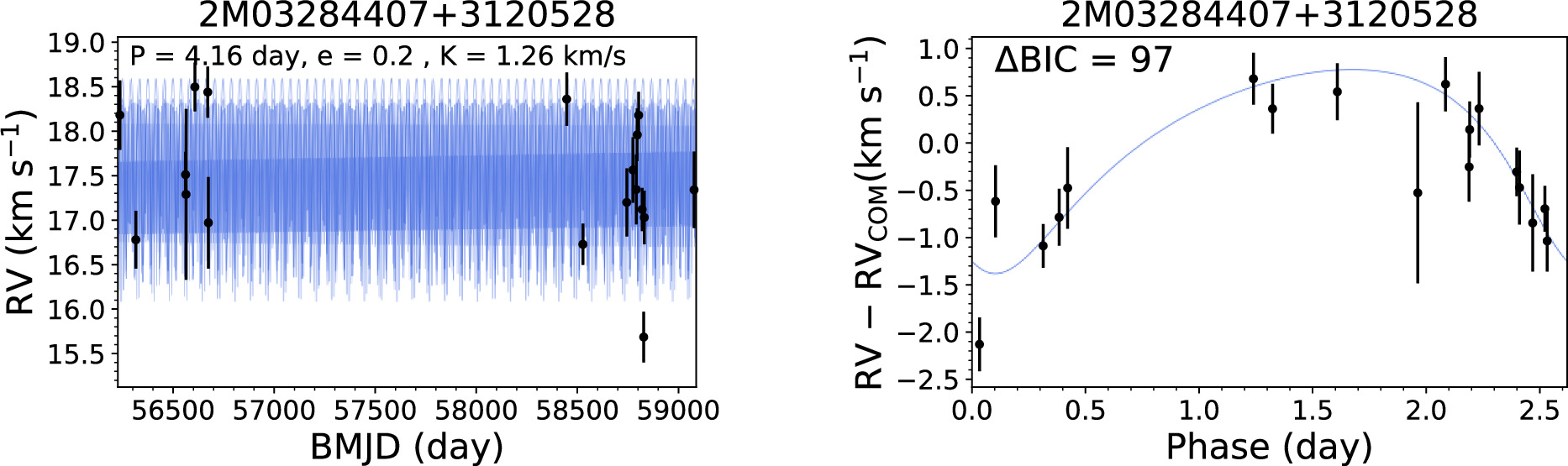