


Abstract
The citizen Continental-America Telescopic Eclipse (CATE) Experiment was a new type of citizen science experiment designed to capture a time sequence of white-light coronal observations during totality from 17:16 to 18:48 UT on 2017 August 21. Using identical instruments the CATE group imaged the inner corona from 1 to 2.1 RSun with 1 43 pixels at a cadence of 2.1 s. A slow coronal mass ejection (CME) started on the SW limb of the Sun before the total eclipse began. An analysis of CATE data from 17:22 to 17:39 UT maps the spatial distribution of coronal flow velocities from about 1.2 to 2.1 RSun, and shows the CME material accelerates from about 0 to 200 km s−1 across this part of the corona. This CME is observed by LASCO C2 at 3.1–13 RSun with a constant speed of 254 km s−1. The CATE and LASCO observations are not fit by either constant acceleration nor spatially uniform velocity change, and so the CME acceleration mechanism must produce variable acceleration in this region of the corona.
Export citation and abstract BibTeX RIS
1. Introduction
The inner corona is notoriously difficult to study, but it is the region where coronal mass ejections (CMEs) are accelerated. Space-based observations of CMEs using Thompson scattered white-light data are limited to heights above 3.1 RSun, and here CME material usually shows a constant speed or deceleration (Sheeley et al. 1999). Measurements in the inner corona can be made using narrowband filter images or X-ray imaging (Alexander et al. 2002; Gallagher et al. 2003; Reva et al. 2017; Seaton & Darnel 2018), but these observations are usually limited to large, rapid CMEs and may be biased by the temperature response of the particular observed radiation. Ground-based observations have been made in white-light (St. Cyr et al. 1999; Mancuso 2007) but these are limited by the higher scattered light background produced by the Earth's atmosphere, and have lower spatial resolution than space-based observations of the region (Elmore et al. 2003). In all cases spatial features of the CME (usually the leading edge) are tracked through an image sequence, and the kinetics of the eruption are inferred from the resulting time–height graph and its derivatives.
White-light observations during a total solar eclipse provide another opportunity to measure the acceleration of CMEs in the inner corona. The likelihood of a CME happening during any total eclipse is low, but CMEs did occur in both the 2008 and 2012 total solar eclipses (Pasachoff et al. 2009, 2015). The 2017 total solar eclipse presented a unique opportunity (Hudson et al. 2011), and the Citizen Continental-America Telescopic Eclipse (CATE) Experiment was developed to exploit this opportunity (Penn et al. 2017). The experiment provided identical sets of equipment to a diverse set of trained volunteer observers and collected a long time-sequence of white light images of the inner corona.
We describe in detail the Citizen CATE Experiment and discuss the CME acceleration measurements provided by a selection of the data. In Section 2 we discuss the instrumentation used in CATE. Section 3 describes the creation of the volunteer network and Section 4 outlines the training program for these volunteers. In Section 5 we discuss the performance of the CATE network on the day of the eclipse, and in Section 6 we describe the resulting CATE data set and the CME acceleration measurements.
2. CATE Instrument
The CATE instrument was assembled from off-the-shelf components, and an effort was made to minimize the cost of the instrument and to make sure that it was fully portable, while still meeting the science goals of the experiment. In total, the CATE equipment for each site cost roughly US $3500. This cost was reduced for most sites through corporate contributions. We discuss the details of the equipment here for those who may wish to duplicate or improve upon it.
2.1. A Telescope and Filters
The CATE telescope was manufactured by Daystar Filters, LLC; and Daystar donated 60 telescopes to the project. The telescope is an 80 mm aperture refractor with an extremely low dispersion (ED) doublet primary lens. The focal length was 500 mm, producing an f/6.25 system. The optical tube assembly (OTA) included a 2'' rack and pinon Crayford focuser with rack and pinion assist and a locking screw. A 2'' to 125 converter and a Baader C-mount to 125 camera adapter were used to insert the CATE camera at prime focus. The OTA was mounted into the telescope mount with a dovetail foot plate. For observations during the partial phase of the eclipse, a full-aperture white light solar filter from Thousand Oaks (S4250) was used at all sites. Several of these filters were cross-calibrated with the same OTA/camera system.
The ED doublet was found to have some chromatic aberration. To minimize this, two color filters were introduced into the beam. A Yellow #12 and an IR Blocking filter (IRBF1) from High Point Scientific were purchased to limit the effective transmission between 480 and 680 nm. Both filters were 125 and were threaded into the camera adapter.
2.2. Telescope Mount and Tracking Drive
The CATE sites used German Equatorial mounts during the eclipse. In particular, a CG4 tripod mount from Celestron, Inc was used; Celestron donated 60 of these mounts to the CATE project. With the CATE OTA and camera system, only a small counterweight was needed to balance the system. On the CG4 a small Televue solar pointer was mounted at the location for the decl. drive, and the R.A. motor from the CG4 dual axis motor drive kit was installed on all the mounts to track the Sun during the eclipse. The R.A. motor was powered with 4 D-cell batteries. The R.A. motor control box allowed the CATE volunteers to make fine pointing adjustments in R.A., while a slow motion manual control was used to make pointing adjustments in decl.
2.3. CMOS Camera
In the years leading up to 2017, different cameras were examined to determine which would be an optimal choice for the CATE project. The camera FOV, pixel size and cost were considered. In 2016 the Point Grey Grasshopper USB3 5 Mpix monochrome camera model GS3-U3-51S5M-C was used at several sites in Indonesia. The detector, a Sony IMX250 CMOS array with a global reset was found to be superior to the array used in the 2015 Faroe Islands eclipse project (Penn et al. 2017). The camera was the most expensive element of the CATE instrument, and unfortunately no corporate sponsor was found to provide the camera. The CATE camera transferred data to a control laptop computer along a USB3 cable, and was also powered by the laptop using the USB3 port. Camera parameters including camera temperature were monitored, and camera communications including exposure control for the calibration images were sent along the USB3 line.
2.4. Arduino
As in the 2016 Indonesian eclipse, a hardware exposure control signal was provided to the camera through the GPIO port for the observations taken during totality. A set of 8 exposures (0.4, 1.3, 4.0, 13, 40, 130, 400 and 1300 ms) was used during the totality sequences, although at many sites the whole camera FOV was saturated in the 1300 ms exposure.
In addition to providing a hardware exposure trigger, the CATE Arduino packages also contained a Global Positioning System (GPS) timing board from ITEAD Royal Tek, model number IM120417017, along with a GPS antenna from Banana Robotics, model number BR010312. The GPS board was mounted in the Arduino Box and connected to the Arduino Uno Rev 3 CPU card. The MathWorks MATLAB SolarEclipseApp software package communicated with the GPS board and data strings received from the board were relayed to the control laptop via the USB2 cable. During the calibration procedures, the Arduino passed GPS strings from this board to the CATE laptop for two purposes: (1) the GPS location of the observing site was recorded, and (2) the GPS timing information was compared with the laptop timing so that the start time of each exposure from all the CATE sites could be converted to a uniform GPS time.
The Arduino operated on power from the CATE laptop using a USB2 cable. The GPIO cable interface to the Arduino digital output pins was custom made for all the CATE sites, and the Arduino packages were installed into modified Arduino project boxes.
2.5. Laptop
The CATE laptops were required to run the operation software, power the CATE camera and Arduino, and store and backup the CATE data, while operating on only battery power if necessary. At least one USB3 port was needed to communicate with the CATE camera. Enough RAM was needed to support the data collection software and enough processing power was required to provide some near real-time display capability while the camera data was being written to disk. A backlit keyboard was preferred to help users needing to type during the dark conditions at totality. The disk write access speed needed to be fast enough so as to not limit the data collection, and finally all of this needed to cost very little, since unfortunately no corporate sponsors were found to supply laptops to the project.
A laptop from Acer (Aspire E15 E5-575G-527J) was found to satisfy most of these requirements. It included a dual-core Intel i5 processor running at 3.1 GHz, operated at 64 bits, and included a solid state drive which had data write speeds that were faster than other laptops without solid state drives. The laptops were augmented with a second 8 Gb RAM card (Ballistix BLS8G4S240FSD) bringing the total laptop RAM up to 16 GB. The laptops used Windows 10 operating system.
2.6. Software
The CATE calibration and data collection procedures were written in MATLAB, by Mathworks, Inc. Mathworks was a CATE corporate sponsor and donated software, funds and licenses for CATE volunteers; additionally, three CATE volunteer observers were Mathworks employees.
Following the 2016 Indonesian eclipse, a brainstorming session was held where the software used during the 2016 eclipse was evaluated, and ideas for a better software package were developed. Key issues were identified, including the difficulty of using the Indonesian GPS package and the focus problems at several Indonesian sites, and particular strategies were developed to minimize these problems for the 2017 eclipse.
The 2017 MATLAB software package presented each volunteer with a graphical user interface (GUI) on which several tabs could be selected. These tabs stepped sequentially through the GPS Data collection, Instrument Setup, Alignment, Focus, Calibration and Totality observations procedures. The GUI enabled multi-threading to utilize both laptop processing cores. A more complete description of each of these steps is presented in Section 4.1 below.
2.7. Miscellaneous
In addition to these main components, the equipment at each CATE site included a few miscellaneous components. During several tests in the summer in Tucson, when the telescope was taking sky flats and the camera body was exposed to direct sunlight, the camera temperature reached 76°C. Communication between the camera and the laptop was lost as the camera overheated, exceeding its 50°C maximum recommended operating temperature. A small battery-powered cooling fan was mounted on the CG4 tripod blowing air across the camera body. More than 10°C of cooling was achieved this way and allowed stable camera operation.
For 2017 eclipse observing locations lacking a power source, the CATE equipment was designed to run for 3 hr on laptop batteries, however several volunteers used external battery power sources to avoid any trouble caused by low battery power on the CATE laptop.
Finally, in order to backup the files immediately after totality, each site was equipped with two USB memory sticks with at least 16 GB capacity each. Two backup copies of the calibration and science data were made directly after totality at each site using these sticks.
3. CATE Volunteer Network
The Citizen CATE Experiment was made possible only through volunteer contributions. The volunteer group was structured into three categories: the CATE site volunteers who would collect eclipse data on August 21 (see Table 1), the CATE state coordinators who identified and coordinated the site volunteers in each state along the path of totality, and the CATE trainers, who helped to develop the CATE observing protocol and then educated the CATE site volunteers and provided feedback to them during pre-eclipse testing. Often a particular individual filled more than one role in the CATE team.
Table 1. CATE Network Sites
| Site | Predicted Start | Predicted End | Approx. Location | Approx. Long. | Approx. Lat. |
|---|---|---|---|---|---|
| cate17-001 | 17:16:06 | 17:18:04 | Lincoln County, OR | −123.87 | 44.83 |
| cate17-002 | 17:17:20 | 17:19:15 | Salem, OR | −123.03 | 44.93 |
| cate17-002b | 17:17:33 | 17:19:32 | Jordan, OR | −122.72 | 44.70 |
| cate17-003 | 17:18:16 | 17:20:17 | Detroit, OR | −122.17 | 44.72 |
| cate17-004 | 17:19:35 | 17:21:38 | Madras, OR | −121.14 | 44.67 |
| cate17-005 | 17:20:59 | 17:23:01 | Fossil, OR | −120.15 | 44.73 |
| cate17-006 | 17:22:20 | 17:24:20 | Mt Vernon, OR | −119.08 | 44.41 |
| cate17-006b | 17:22:30 | 17:24:28 | Canyon City, OR | −118.96 | 44.38 |
| cate17-007 | 17:23:00 | 17:25:07 | Prairie City, OR | −118.62 | 44.58 |
| cate17-008 | 17:24:24 | 17:26:33 | Malheur County, OR | −117.59 | 44.42 |
| cate17-000 | 17:25:17 | 17:27:23 | Weiser, ID | −116.97 | 44.26 |
| cate17-000b | 17:25:17 | 17:27:23 | Weiser, ID | −116.97 | 44.26 |
| cate17-009 | 17:25:17 | 17:27:23 | Weiser, ID | −116.97 | 44.26 |
| cate17-010 | 17:26:46 | 17:28:50 | Crouch, ID | −115.97 | 44.12 |
| cate17-011 | 17:28:23 | 17:30:36 | Stanley, ID | −114.88 | 44.14 |
| cate17-012 | 17:30:20 | 17:32:33 | MacKay, ID | −113.61 | 43.91 |
| cate17-013 | 17:31:18 | 17:33:28 | Howe, ID | −113.00 | 43.78 |
| cate17-012b | 17:32:56 | 17:35:13 | Annis, ID | −111.97 | 43.75 |
| cate17-014 | 17:33:05 | 17:35:22 | Rexburg, ID | −111.88 | 43.82 |
| cate17-015 | 17:34:26 | 17:36:37 | Tetonia, ID | −111.10 | 43.82 |
| cate17-p001 | 17:34:26 | 17:36:39 | Clawson, ID | −111.08 | 43.79 |
| cate17-016 | 17:35:18 | 17:37:37 | Kelly, WY | −110.53 | 43.63 |
| cate17-017 | 17:36:51 | 17:39:08 | Dubois, WY | −109.62 | 43.54 |
| cate17-018 | 17:38:19 | 17:40:40 | Fremont County, WY | −108.76 | 43.20 |
| cate17-018b | 17:38:58 | 17:40:59 | Arapahoe, WY | −108.49 | 42.96 |
| cate17-019 | 17:39:06 | 17:41:19 | Riverton, WY | −108.35 | 43.01 |
| cate17-020 | 17:40:48 | 17:43:10 | Arminto, WY | −107.34 | 43.11 |
| cate17-021 | 17:42:35 | 17:45:01 | Casper, WY | −106.35 | 42.81 |
| cate17-022 | 17:42:39 | 17:45:04 | Casper, WY | −106.32 | 42.85 |
| cate17-023b | 17:45:09 | 17:47:36 | Glendo, WY | −104.98 | 42.47 |
| cate17-023 | 17:45:42 | 17:47:59 | Guernsey, WY | −104.76 | 42.29 |
| cate17-022b | 17:46:18 | 17:48:46 | Jay Em, WY | −104.36 | 42.46 |
| cate17-024 | 17:47:33 | 17:49:55 | Agate, NE | −103.73 | 42.42 |
| cate17-025 | 17:48:56 | 17:51:26 | Alliance, NE | −103.01 | 42.12 |
| cate17-026 | 17:51:30 | 17:54:02 | Hyannis, NE | −101.73 | 41.78 |
| cate17-027 | 17:53:26 | 17:55:59 | Tryon, NE | −100.79 | 41.52 |
| cate17-028 | 17:55:47 | 17:58:13 | Broken Bow, NE | −99.64 | 41.40 |
| cate17-029 | 17:57:33 | 18:00:08 | Ravenna, NE | −98.83 | 40.99 |
| cate17-030 | 17:59:44 | 18:02:18 | Sutton, NE | −97.85 | 40.61 |
| cate17-031 | 18:02:17 | 18:04:52 | Beatrice, NE | −96.71 | 40.25 |
| cate17-032 | 18:03:32 | 18:06:08 | Pawnee City, NE | −96.15 | 40.11 |
| cate17-033 | 18:05:02 | 18:07:36 | Hiawatha, KS | −95.52 | 39.85 |
| cate17-034 | 18:05:38 | 18:07:21 | Atchison, KS | −95.56 | 39.56 |
| cate17-035 | 18:08:01 | 18:10:36 | Lawson, MO | −94.24 | 39.41 |
| cate17-036 | 18:10:27 | 18:13:06 | Marshall, MO | −93.17 | 39.11 |
| cate17-037 | 18:12:20 | 18:14:58 | Columbia, MO | −92.34 | 38.93 |
| cate17-038 | 18:14:34 | 18:17:02 | Hermann, MO | −91.41 | 38.70 |
| cate17-039 | 18:16:44 | 18:19:22 | Hillsboro, MO | −90.55 | 38.26 |
| cate17-040 | 18:18:35 | 18:21:15 | McBride, MO | −89.86 | 37.86 |
| cate17-040b | 18:20:03 | 18:22:39 | Union Country, IL | −89.34 | 37.55 |
| cate17-041 | 18:20:02 | 18:22:40 | Carbondale, IL | −89.25 | 37.70 |
| cate17-p002 | 18:20:06 | 18:22:44 | Carbondale, IL | −89.21 | 37.71 |
| cate17-042 | 18:20:17 | 18:22:57 | Makanda, IL | −89.18 | 37.60 |
| cate17-042b | 18:21:58 | 18:24:37 | Golconda, IL | −88.51 | 37.36 |
| cate17-043 | 18:22:24 | 18:25:04 | Burna, KY | −88.37 | 37.23 |
| cate17-044 | 18:24:52 | 18:27:32 | Hopkinsville, KY | −87.43 | 36.81 |
| cate17-044 c | 18:24:55 | 18:27:34 | Hopkinsville, KY | −87.41 | 36.82 |
| cate17-044b | 18:25:39 | 18:28:17 | Guthrie, KY | −87.16 | 36.64 |
| cate17-045 | 18:26:14 | 18:28:53 | Adairville, KY | −86.85 | 36.67 |
| cate17-047b | 18:27:31 | 18:29:08 | Nashville, TN | −86.83 | 36.12 |
| cate17-046 | 18:28:03 | 18:30:41 | Hartsville, TN | −86.16 | 36.38 |
| cate17-047 | 18:29:43 | 18:32:15 | Cookeville, TN | −85.50 | 36.17 |
| cate17-048 | 18:31:47 | 18:34:26 | Spring City, TN | −84.80 | 35.67 |
| cate17-049 | 18:32:58 | 18:35:34 | Madisonville, TN | −84.31 | 35.54 |
| cate17-050 | 18:34:27 | 18:37:05 | Andrews, NC | −83.81 | 35.20 |
| cate17-051 | 18:37:12 | 18:39:49 | Clemson, SC | −82.83 | 34.67 |
| cate17-052 | 18:39:20 | 18:41:48 | Greenwood, SC | −82.16 | 34.20 |
| cate17-053 | 18:41:29 | 18:44:04 | Lexington, SC | −81.20 | 33.98 |
| cate17-054 | 18:43:03 | 18:45:27 | Orangeburg, SC | −80.84 | 33.49 |
| cate17-055 | 18:44:31 | 18:47:06 | Cross, SC | −80.13 | 33.38 |
| cate17-055b | 18:46:27 | 18:48:25 | Isle of Palms, SC | −79.77 | 32.79 |
| cate17-056 | 18:46:11 | 18:48:45 | Bulls Bay, SC | −79.56 | 33.03 |
Note. The six sites used in the present analysis of the CME outflow are shown in bold text. Sites with cloudy conditions or instrumental difficulty are shown in italics. Predicted lunar limb corrected totality start (C2) and end (C3) times are shown (Jubier 2017). Truncated latitude and longitude coordinates are shown for reasons of privacy, and may be up to 1 km away from actual CATE observing site.
3.1. State Coordinators
A set of coordinators was identified, one from each state crossed by the 2017 path of totality. Faculty mentors from the universities participating in the 2016 eclipse formed the core of this group of state coordinators and organized efforts in Wyoming, Illinois, Kentucky and South Carolina. To this core group individuals from Oregon, Idaho, Nebraska, Missouri, and Tennessee were added to build a group of nine CATE state coordinators. These coordinators included additional university faculty, high school teachers and amateur astronomers, and they participated voluntarily in the program. Frequent meetings of the state coordinators were held with teleconferencing, and these state coordinators then met with the CATE site volunteers via phone, teleconference or in-person. The state coordinators and trainers provided input into the CATE equipment selection, software control and data analysis.
3.2. Observing Location Selection
Initially a set of observing locations for the 2017 eclipse was determined using an equally spaced set of locations across the path of totality from the Pacific to Atlantic coasts. Google maps was used to identify school or park locations with easy access that were close to the centerline at the desired spacing. During a second round of analysis the local times for the eclipse contacts were used to determine if the site locations needed to be adjusted. These second-level sites were then presented as suggestions to the CATE state coordinators. The coordinators used their knowledge of the locations, local weather patterns, and the experience of their site volunteers to refine the CATE observing sites a third time. With this optimal set of locations, the CATE coordinators and site volunteers then attempted to get permission to use these sites during the day of the eclipse; some of the sites were relocated a fourth and final time depending on the ability of the volunteers to observe from the area. Using this iterative procedure, the CATE observing sites were established using local knowledge to maximize the likelihood of obtaining excellent eclipse observations.
4. CATE Observing Procedures and Training Program
The CATE training program for the 2017 eclipse built on progress made through observations and training carried out over the previous two years. An initial observation guide was developed for the 2015 March 28 eclipse where the first CATE volunteer traveled to the Vagar airport in the Faroe Islands to collect coronal data using a CATE prototype telescope system. The trip was a proof of concept that a dedicated volunteer with no previous astrophotography experience could be trained on the Citizen CATE observation procedures in a relatively short period of time and successfully gather coronal data during a total solar eclipse. Despite poor site conditions with rain and clouds, 800 frames of calibration data during the partial phases of the eclipse as well as 37 images of the inner corona during totality were collected.
Procedures were further refined leading up to the 2016 eclipse when four student and mentor teams from CATE partner institutions at the University of Wyoming, Southern Illinois University Carbondale, Western Kentucky University, and South Carolina State University observed the 2016 March 9 total solar eclipse from 4 ground locations in Indonesia. A fifth volunteer team observed the eclipse from a cruise ship. The students had attended training prior to the trip and practiced with their mentor and observation teams at their home institutions. The groups used a MATLAB Solar Eclipse Application developed in cooperation with MathWorks. The experience gained in Indonesia by the teams proved critical in training the students and mentors as this was the first eclipse for each of the ground based teams. Four out of the five sites were able to collect eclipse data with one site being clouded out. The observations allowed teams to test the observing procedure and provide valuable feedback that was integrated into the procedures for the 2017 eclipse event.
4.1. Procedure
Solar and lunar observation procedures were designed in order to give the CATE 2017 volunteers a basic understanding of equipment and an introduction to the procedure at workshops held in several states across the path of totality. The procedure served as a guide for all practice sessions and ultimately the observations during eclipse. Procedures were split into five sections: Setup, Preliminary Data, Eclipse, Data Backup and Quick look. Throughout the procedures, the amount of time allotted for each task was listed as a guideline to keep volunteers on schedule so they were prepared to take totality data at the time of the eclipse. With perfect sky conditions and no instrument problems, the procedure took approximately 2.5 hr to perform.
4.1.1. Setup
Volunteers started by first setting up and leveling the Celestron CG-4 GEM tripod and aligning the mount. They were instructed how to align the telescope using the Rackley Method (Rackley 2017) as well as a more traditional method of day time alignment with a compass, taking into account magnetic north deviation for their location. Cameras were installed with a procedure so that the camera rotation was similar among all the sites, accounting for which sites observed from different sides of the polar axis. Volunteers balanced the mount, turned on tracking, connected all equipment, and set the initial focus before the MATLAB Solar Eclipse App was started.
4.1.2. GPS
Tabs at the top of the Solar Eclipse App guided volunteers through each step of the observation. In the first tab, the user would verify the GPS card in the Arduino electronics box was connected and passing data to the computer properly. The user then collected a two-minute sequence of GPS data, which recorded time and location. Finally, a second tests was run to verify that the Arduino electronics box was sending the proper timing strobes to the camera hardware trigger input.
4.1.3. Alignment
The Alignment tab allowed volunteers to set the exposure value so they could clearly see the solar disk through the ND filter without oversaturating, and then center the Sun in the camera frame using a combination reticle of a crosshair and a circle that matched the solar diameter. Volunteers first centered the image, and then fine-tuned the camera rotation by observing the image movement on the CATE camera while R.A. or decl. adjustments are made. Proper rotation was achieved when the image moved horizontally when the R.A. screw was adjusted and vertically when the decl. screw was adjusted.
The volunteers then used the live solar image to adjust the polar axis of the CG-4 mount. Fine adjustment of the polar alignment is accomplished by going to the Focus tab and observing the drift of the solar limb or a sunspot. This tab allowed volunteers to zoom in on a region of interest (ROI) and observe small image drifts. Because the R.A. drive tracked at a standard sidereal rate, proper motion of the Sun would result in an eastward drift of about 004 per second (about 0.03 pixels per second). Volunteers were asked to adjust the mount until the drift was less than 12 per second (about 1 pixels per 1.3 s) to ensure minimal image smearing for the longest exposures planned for the totality phase of the eclipse.
After the volunteers completed the camera rotation and polar axis alignment steps, they were asked to take two data sets to quantify their alignment results. First, a sequence of 100 images (one image per second) was recorded with the mount R.A. tracking running to determine polar alignment accuracy. A second sequence of 100 images was recorded with the R.A. tracking off to determine the direction of geocentric west on the camera pixels in order to test the accuracy of the camera rotation. This data was analyzed during practice sessions to provide support to the CATE teams, and were analyzed on the day of the eclipse as a data quality indicator.
4.1.4. Focus
The next setup step was to finely adjust the telescope focus. This was done by observing a ROI (typically on the lunar limb) on the camera display while manually adjusting the focus. A quantitative measure of focus quality (determined from the intensity gradient of the image) was displayed and allowed volunteers to verify their focusing. This was of significant assistance if the site was performing the focus procedure during cloudy conditions that obscured features on the Sun or the lunar limb. Once the best focus was achieved, the focus was manually locked with a set screw and a snapshot image of the focus ROI was saved to disk.
On all tabs in the procedure, there was a live camera temperature monitor. Due to the high heat in some locations during practice sessions, the camera would occasionally overheat and behave erratically. Although camera operations were specified by the manufacturer only up to 50°C, during tests we found that the camera functioned normally while the internal temperature was below 65°C. The temperature monitor display in the app was set to turn red over 65°C, alerting volunteers to cool the camera using a simple fan and shade. At critical times in the procedure such as the fine focus procedure, the fan was temporarily turned off to minimize vibrations that could affect image quality. There were no failures resulting from overheating cameras on the day of the eclipse.
4.1.5. Calibration
Calibration data required for each site consisted of GPS location and timing, drift data, and a set of flat and dark frames. These were taken by the user on the GPS, Drift, and Calibration tabs.
Flat and dark frames were collected by going to the Calibration tab. For flat images the telescope was rotated 90° away from the Sun to a clear patch of sky, the solar filter was removed and the user selected "Log Data (Sky FLATS)," in the app. A sequence of 100 images (collected at 1 image per second) were stored to the disk.
Dark images at a variety of exposures needed to be collected with the telescope dust cover on the front of the aperture. A sequence of 100 dark images at the same exposure as the sky flats were stored to disk, and another sequence of 100 frames at the same exposure as the drift test solar images. In each case the software stored the required exposure values and the volunteer did not need to enter the value. The final sequence of darks, called Totality darks, was taken using the same hardware triggering as employed for the totality images. This was a sequence of 8 different exposures, and the software cycled through these exposures to collect 100 frames again, spanning 12 complete exposure cycles.
The calibration data was ideally collected prior to totality, however volunteers were given the option to collect data after totality if time became an issue.
4.1.6. Totality
Volunteer teams following the nominal procedure schedule would have 25 minutes to wait for totality after completing the initial procedures. During this time volunteers kept the telescope tracking on the partial phase of the eclipse. Teams had two or more members with each member assigned to a specific task at the start and end of totality. At the start of totality, one volunteer would remove the solar neutral-density filter from the telescope and the other would begin recording totality images. The app displayed a live view of totality that the team used to verify the Sun was centered properly, the exposures were being triggered, and it also displayed a running count of the number of frames captured. The totality sequence averaged 4 frames per second or about 600 totality frames for each site. In the event of cloudy skies, teams collected totality data at the expected time of totality; data collection was to occur regardless of whether or not the team members could see totality so that the team would not have to scramble and start taking data if the clouds suddenly parted.
Once totality was over, teams stopped the data collection, and immediately copied the data to external USB flash drives. Depending on the write speed of the device, this could take up to 30 minutes since each site collected about 12 GB of data. As soon as backups were complete, volunteers proceeded to the "Quick Look" tab to produce a high-dynamic range (HDR) image that was created by combining eight single exposures. The HDR image as well as a few calibration files were uploaded to a website for inspection, and one of the USB drives with the full data set was then mailed to the PI. Each site volunteer reported to their team leader via text or phone about the success at their site so a project-wide status could be determined nearly in real-time.
4.2. Workshops
CATE coordinators hosted twelve training workshops from April 22 through May 28. At the workshops the CATE equipment was distributed to the site volunteers. State coordinators, teaming with a CATE student, guided the site volunteers through the solar observing sequence. In some states with widely distributed volunteers, two workshops were held. TN and KY combined their workshops into one location, and a workshop was held in Tucson AZ for several groups from the southwest. Overall workshop participation was good with 130+ participants attending, representing 62 out of the 70 observation sites.
The workshops shared a set of several goals, and emphasized the safety issues involved in observing the Sun. Many of the Citizen CATE sites were in public areas where the citizen CATE teams would be the eclipse guides for the public. Teams were instructed on safe public solar viewing as well as how to develop their site-specific safety plan. Teams were encouraged to identify members who would work with the public exclusively so the other team members could concentrate on running the telescope. Teams worked through the solar procedure first indoors on a test image, and then outdoors on the Sun. Test data collected at the workshops were uploaded to a common website in the same way it would be done in summer practices and during the August eclipse.
4.3. Summer Practice
Due to the time-critical nature of the eclipse observations, it was important that teams practice and become proficient using the equipment. The goal of the workshops was to familiarize teams with the equipment and get them to the point that they could take part in practice observation campaigns as well as practice on their own. Volunteers were then asked to begin day and night time observations and upload data of the observations for evaluation. Participating in both day and night time observations prepared teams by imaging the full disk of the Sun during conditions similar to partial eclipse phases, and imaging the moon, which provided a target of similar brightness to the solar corona.
In addition to independent practice, several network-wide training dates were established. The main purpose of these practice runs was for the teams to learn how to complete observations in a timely manner, often in less than ideal conditions. Practices also revealed issues with the procedures and allowed the CATE team to provide feedback to volunteers on the quality of their data.
Table 2 lists several parameters measured during the network-wide summer training dates. Team participation in training sessions was at or above 50% for the first three training sessions and decreased during the last two sessions. The average focus quality improved after the first two training sessions and then decreased slightly again. The polar alignment for the sites, as measured by the solar image drift while the telescope was tracking, improved by a factor of two through the summer. The camera rotation, as measured by the angle of the solar image drift during the tracking off sequence (270° is ideal), improved initially and remained good. Finally, during the last three practice sessions, the ability of volunteers to center the solar image was measured, and this also showed improvement with time.
Table 2. Analysis of Data from 2017 CATE Network Practice Sessions and Eclipse Data (bold values)
| Date | # of Sites | Focus (arb.) | Drift (pix sec−1) | Drift Angle (deg) | Image Offset (pix) |
|---|---|---|---|---|---|
| Jun 24 | 37 | 0.051 | 0.37 | ⋯ | ⋯ |
| Jul 08 | 36 | 0.051 | 0.33 | 268.1 | ⋯ |
| Jul 22 | 34 | 0.056 | 0.23 | 270.8 | 19 |
| Aug 05 | 15 | 0.055 | 0.20 | 270.2 | 11 |
| Aug 12 | 21 | 0.053 | 0.18 | 270.2 | 16 |
| Aug 21 | 50 | 0.056 | 0.22 | 270.0 | 17 |
Note. Larger "focus" values represent better image quality, and the experiment goal was to align the "drift angle" to exactly 270 0. Smaller values of "drift" and "image offset" are better than larger values.
Download table as: ASCIITypeset image
Significant improvements to the solar eclipse app were also made at this time. Required updates to Arduino code and the app were pushed out to state coordinators who beta tested the changes and quickly provided feedback to the core team. Once the code was determined to be stable, new versions were made available to all volunteers. Since the workshops included instruction on uploading Arduino code to the microcontrollers as well as basic computer configuration and app installation, the majority of the teams were able to quickly adapt the changes into their own computers and start using new procedures.
5. The 2017 August 21 Eclipse
5.1. CATE Sites: Locations and Timing Calibration
The GPS board received timing and location information. On the "GPS" tab of the SolarEclipseApp software, the CATE volunteers selected a communications channel and viewed the GPS strings in a live display. Each site was instructed to run a GPS data acquisition routine during their pre-eclipse activities. About 1300 GPS strings were collected and saved to the file during roughly 120 s of time for each site. These text files were analyzed to determine the site latitude and longitude, and to determine the timing offsets between GPS time and each laptop time.
5.1.1. Site Location
For each CATE site, about 118 location strings were collected with the GPS equipment; only one CATE site had no valid GPS strings in the recorded file, and the site coordinates were entered manually based on a Google Maps location. In all cases the GPS location strings were recorded in a dddmm.mmmm format, with ddd listing the degree value, and mm.mmmm listing the minute and decimal minute values of the GPS location. For privacy reasons Table 1 does not list the detailed locations for each site. Based on the standard deviation of the recorded GPS location strings, the internal precision is very high, less than 1 m. A better error estimate can be made using the GPS locations for Sites 000, 000b and 009, all of which were located near the southeast corner of the athletic field of Weiser High School in Weiser Idaho. Based on the GPS data collected from these three sites the estimated CATE site location accuracy is about +/−30 m (+/−00003).
5.1.2. Site Timing
During initial testing it was found that tagging the eclipse exposures with a time from the GPS Arduino shield resulted in significant overhead, slowing the data collection. Instead we decided to tag each image with a CPU time (which was much faster) and then to compute the offset between CPU time and GPS time for each laptop in the network. By using GPS data collection to compute the offset Δt, we could convert from CPU time to GPS time with tGPS = tCPU + Δt.
A total of 23,800 GPS timing strings were collected across the 70 sites. On average these timing strings were collected 106 minutes before totality; for nine sites the strings were collected more than 180 minutes before totality, and for six sites the timing information was collected up to 46 minutes after totality. The computed values for Δt ranged from 300 s behind UT to 85 s ahead of UT, with a median value of 2.63 s behind UT. Without computing this value, there would be significant errors when combining data from the CATE sites.
There are errors expected in both the tCPU and Δt terms, and so there is an error in the tGPS term also. Errors in tCPU arise from drift in the laptop clock. This was measured in several laptops before the eclipse, and the drift rates averaged 60 ms per hour. Occasionally jumps of 120 ms were seen in these timing tests. We estimate this error as 90 ms. Errors in Δt can arise from variations in the signal transfers from the GPS shield card to the Arduino board, from the Arduino board to the USB port, and from the USB port to the Matlab code. During the day of the eclipse, 6 sites collected two sets of GPS timing strings. The differences in the two values of Δt calculated for these laptops ranged from 3 to 46 ms, with a median value of 11 ms. Here we use 11 ms for the error. With these values, the formal error in tGPS can be calculated to be 91 ms; so we approximate the timing error for any exposure on any laptop during the CATE experiment at 100 ms.
5.2. Observer Performance
CATE site volunteers experienced a variety of weather conditions along the path of totality. Conditions were mostly clear on the west coast, and the skies remained clear, except for a few places, along the eclipse path until eastern Nebraska. A patch of clouds was found from eastern Nebraska through western Missouri, and then mostly clear conditions prevailed again until Illinois and western Kentucky. Partly cloudy conditions challenged CATE observers along the path of totality from Kentucky to the east coast.
The last row of Table 2 shows the focus, polar alignment, camera rotation, and image alignment specifications for CATE observers on the eclipse day, August 21. In order to distinguish cloudy sites from clear sites, the image intensity of the tracking-on and tracking-off time sequences was used. (It is likely that there is useful data from the sites with lower or highly variable image intensity, but those have not yet been examined.) Stable image sequences with the CG4 mount tracking the Sun were collected from 46 sites, and good image sequences with the CG4 mount turned off (and the solar image drifting across the camera) were collected from 50 CATE sites.
The image focus values obtained on the eclipse day matched the best focus values from any practice session. The quality of the mount's polar alignment is measured by the amount of solar image drift during 100 s of tracking. To ensure minimal image smearing, a tracking drift of less than 1 pixel in 1.3 s was the goal for the polar alignment error (0.77 pixels per second). Through all of the practice sessions listed in Table 2 this goal was met, and the eclipse day drift value (0.22 pixels per second) easily met the goal. The camera angle adjustment on average was the best recorded during the summer, although five sites were rotated 180° away from the optimal orientation. Finally, the image centering achieved by the CATE volunteers on eclipse day was good.
5.3. Camera Calibration Images
Standard dark and flat images were taken during the pre-totality operations at each CATE site. The dark images for the totality sequences were taken using the same Arduino hardware camera triggering that was used during totality; darks were taken in a sequence of 8 exposure times, consisting of 0.4, 1.3, 4.0, 13, 40, 130, 400 and 1300 milliseconds. A sequence of 100 darks was saved to the laptop disk drive, consisting of 12 complete 8 exposure sequences and four additional frames.
A close examination of the hardware triggered exposures (the totality images and the totality darks) shows some evidence of random intensity jumps. These do not seem to be sticky bits, but seem to be deviations in the exposure time caused by the timing signals from the Arduino. In the dark frames where the signal level is about 660 counts, the jumps can be about 30 counts, and only affect one frame in the sequence of 12. This suggests these trigger errors can cause intensity errors of about 1.3%. In the totality images the signals are generally 7000 counts or higher, and about 600 images are co-added to produce an HDR frame; we estimate these trigger errors can introduce intensity errors of 0.017%.
The flat field exposures and the associated darks for the flats were triggered with a software timing trigger, and neither of these images show the random variations seen in the other calibration data.
6. Radial Acceleration of CME Material
The 110,000 image CATE data set is unique, and thus requires a novel analysis process. For this paper we have selected a set of the observations from just six sites (CATE-005, 000, 011, 012, 014 and 018) and discuss the analysis and scientific results from them. The times covered by these images ranges from 17:22:02 to 17:39:30 UT.
6.1. A Image Alignment
Alignment of the CATE data is challenging. Among the totality exposures frames from one site, motion occurs as (1) the telescope does not exactly track the Sun, (2) the moon moves against the solar corona and (3) the Sun moves against the background R.A./decl. coordinate frame. The fourth alignment concern is that the different CATE sites have different image rotation. Since the CATE sites are scattered around the center line of totality, the lunar disk eclipses the solar disk in different ways, leading to a different spatial distribution of atmospheric scattered light. Finally the atmospheric conditions vary from site to site, further complicating stray light contamination.
The general procedure which was used to align this initial science data set was to compute lunar disk position to align each group of 8 sub-exposures and to produce one HDR frame. All of these HDR images from one site were interpolated to a common image center. Solar features were then tracked to determine a second set of offsets, and then all of the HDR images from one site were aligned and summed. Angular cross-correlation functions were computed using an annular region of a spatially filtered version of this HDR image to determine the rotational offsets between each site.
In this set of 6 images, two stars were seen, and were used to further refine the angular and spatial offset alignment, and to orient each image onto an R.A./decl. grid. The two alignment stars (HD 86898 and GM Leo) were also used to measure the image scale from these sites. The stars are 29762 apart, and this produces an image scale of 143 per pixels. The scale variations among these six sites is less than 001 per pixel, attesting to the excellent uniformity in the CATE optics system; solar disk measurements from all the CATE sites also point to uniformity at this level. Unfortunately the stars are not visible in the individual CATE exposures or the first-round HDR images.
6.2. Spatial Filtering and Velocity Measurement
After image alignment, two types of spatial filtering were applied to the CATE images to emphasize the low contrast coronal structures. First a normalized radial gradient filter (Morgan et al. 2006) was used to remove the steep radial intensity gradient from the coronal images. The radial gradient in raw camera counts from the CATE sites shows a brightness variation of a factor of 300 from the limb of the moon to the edge of the FOV. While stray light, atmospheric transmission and equipment variation between these two sites is expected to change the measured coronal intensity, the signals compare very favorably among sites that have clear skies.
The second filter was a combination of box-car averaging and then a simple edge-enhancement Sobel filter. This filtering enhanced coronal fine-scale structures to facilitate feature tracking in the time series. Sample NRGF and Sobel filtered images are shown in Figure 1.

Figure 1. Sample images from CATE site 005. The top figure is the summation of 70 HDR frames aligned and then filtered with a normalized radial gradient filter. The inset on the lunar disk shows a single 1.3 msec exposure from site 005 at full spatial resolution. The bottom figure is an image showing a Sobel filter applied to an 8 pixel smoothed version of the top image.
Download figure:
Standard image High-resolution imageA time sequence of the filtered images reveals a variety of changing coronal features. The most apparent changes occur in along the SE solar limb where material is moving outward through the solar corona. This location corresponds to a CME observed by LASCO SoHO instrument. LASCO height-time plots show that the event had an outflow velocity of 254 km s−1 at the observed heights between 3 and 13 RSun, with an extrapolated start time of 13:55 UT and nearly no acceleration, (−0.2 m s−2) (CDAW Data Center 2019).
The CATE images were divided into sub-images, and spatial cross-correlation was used to determine local image shifts between sequential image pairs. The shift values were divided by the time interval between the images and the spatial scale was used to compute a velocity; both radial and tangential velocity components were computed. Figure 2 shows a grayscale, spatially filtered image of this region of the corona with the computed velocity vectors overlaid on the grayscale. The spatial ROI showing the CME outflow was determined to lie between two prominent and stationary coronal threads. The velocities measured in the CME ROI were then averaged in radial bins of 0.1 RSun; the standard deviation of the mean was also computed for each radial bin.

Figure 2. A sample frame from the CATE time series showing the SE solar limb with a Sobel filter applied. On top of the gray scale are arrows showing the scaled motions of the coronal plasma measured with a cross-correlation technique in the CME region of interest common to all 6 images.
Download figure:
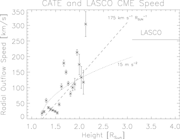
Standard image High-resolution imageThe average radial velocity versus radial distance is shown in Figure 3. Individual points are the radially averaged outflow speeds, the error bars are the standard deviation of the mean for each bin, and a linear fit is shown by the dotted line. The outflow speed measurements from LASCO time–height analysis of the CME leading edge are shown as the horizontal line starting at 3.1 RSun at 254 km s−1 outflow speed.
Figure 3. The radial outflow speed with height, averaged over the coronal mass ejection region of interest. The points represent averages of the radial outflow in bins of 0.1 RSun. The error bars are the standard deviation of the mean for the values in that bin. The CATE data extend from 1.2 to 2.1 RSun, but measurements from LASCO C2 at 3.1 RSun and higher are shown by the horizontal line at 254 km s−1. Two fits to the CATE data are shown: a constant acceleration model of 15 m s−2, and a model showing a spatially increasing velocity with a slope of 175 km s−1 RSun−1. A spatially changing acceleration is required to explain the observed CME velocities.
Download figure:
Standard image High-resolution image
There are two fits to the CATE data which are both extrapolated to a height of 3.1 RSun. First, the dotted line shows a model with a constant acceleration of the CME material; the best fit acceleration is 15 m s−2. The dashed line shows a constant velocity increase with increasing height intervals of 175 km s−1 RSun−1; this represents a changing acceleration with height. Both models assume that the radial velocity equals 0 at a height of 1.2 solar radii. Both models eventually exceed the outflow speed measured by LASCO data, and so the acceleration mechanism must stop or significantly decrease below a height of 3.1 RSun. Using the constant acceleration model, the CME material in the CATE FOV at 2.1 RSun would enter the LASCO C2 FOV at about 19UT; using the other acceleration model the material would enter the C2 FOV slightly earlier. In the C2 movie, CME material continues to stream out of the Sun until after 22UT, so the plasma observed by CATE is certainly associated with the event observed by LASCO.
6.3. Discussion
This analysis of CATE data measures apparent CME plasma velocity by mapping the spatial shifts of many plasma features in the images and averaging these shifts in radial bins. It provides a more flexible method for computing the plasma acceleration than other studies, since only the first derivative is needed, and the velocity (and acceleration) can be mapped across many spatial positions and times. All previous CME kinetic studies measure the changing position of one or two CME features with time, compute the velocity by taking the first derivative of the position, and then compute the acceleration by taking the second derivative of the position.
The CATE data measures the white light corona rather than particular emission lines. Coronal plasma at all temperatures is equally sampled in this data. In the EUV work of Reva et al. (2017) which used TESIS Fe 171 and EIT He 304 images, different parts of the CME that were studied had different temperatures and thus different visibilities. Furthermore, the temperature of the CME regions may change with time, and so tracking features in a sequence of EUV images involves more assumptions than tracking features in a sequence of white light images. With those assumptions, Reva et al. (2017) track two features, the leading and central regions of a CME, and find different velocities and accelerations for those regions. The leading CME region shows a terminal outflow speed of about 400 km s−1, and the central region moves outward more slowly at about 250 km s−1. They attribute the observed kinetics, and the temporal changes of the kinetics to a variety of mechanisms including reconnection, mass drainage and magnetic instabilities.
Like the work of Reva et al. (2017), we measure the CME acceleration not just at the leading edge, but at many locations. The CME in this CATE data has a terminal outflow speed similar to the central region of the Reva et al. CME; they find acceleration values of between −20 and +35 m s−2, similar to our observed accelerations of around 15 m s−2. But unlike that work, we find that the velocity and acceleration of the plasma well behind the CME front is consistent with the leading edge velocity measured by LASCO (which is also measured with white light data). While magnetic reconnection is often discussed as an acceleration mechanism associated with the initiation and leading edge of a CME (Chen 2011), the fact that the trailing plasma observed in this CATE data shows an outflow speed similar to the CME front may provide support for other acceleration mechanisms in this CME, such as magnetic instabilities. This CME may simply exhibit different characteristics from the one studied by Reva et al. (2017), or the assumptions used in the EUV analysis to track features may lead to incorrect velocity measurements for different parts of the CME.
Observations of the solar corona were taken with EUV instruments on the day of the eclipse, for instance with the Proba2 mission and with SUVI. Examining the difference movies from Proba2 at the time of the CATE observations (http://proba2.sidc.be/swap/data/mpg/movies/2017/08/) shows only noise or no signal above a height of about 1.1 solar radii. While the raw Proba2 images (which are not aligned) do show some structures at higher locations, a full analysis of that data set is beyond the scope of this paper. Similarly, SUVI data from the eclipse has not been reduced with the standard pipeline process, and a full analysis of those measurements is again beyond the scope of this paper. Future work comparing the CATE data with these EUV measurements will likely be fruitful, and future analysis of the full CATE data set from all sites will likely reveal more flows in different regions of the solar corona.
7. Summary
The Citizen CATE Experiment was a unique citizen science project. It was funded by a combination of federal, corporate and private contributions, and involved volunteers from middle school students through professional solar astronomers. The volunteers were granted full ownership of the CATE equipment, and several groups continue to use the equipment for educational and outreach projects today.
The data set collected by the Citizen CATE Experiment from the 2017 total solar eclipse is unique. The white light images show coronal material escaping from the Sun during the late phase of a slow CME event which occurred before the eclipse; previous studies report the acceleration of fast CME events by measuring the position of the outwardly moving front as the CME is initiated. We report an acceleration by measuring the velocities of the CME material, which show a change with height in the solar atmosphere. All previous studies directly measure CME position and report an acceleration as the second derivative of their measurements; the CATE data provides a new measurement of the acceleration by showing a change in the CME velocity with spatial position. When the CATE measurements are combined with the LASCO C2 data, it is clear that a uniform acceleration cannot explain the kinetics of this CME, and that the acceleration mechanism must change at different heights in the solar atmosphere.
The CATE team gratefully acknowledges financial and multi-site equipment support from Jen Winter (Daystar LLC), David Garrison (Mathworks, Inc), Corey Lee (Celestron LLC), and Stephen Lauro (colorMaker, Inc). The CATE team appreciates the site equipment support from Rosamond Kinzler of the American Museum of Natural History and from Bill Kloepping. The CATE team acknowledge Research Corporation for Science Advancement award 24174, NASA Cooperative Agreement NNX16AB92A, NASA award NNX17AH76G, and NSF award 1732227. D.W. acknowledges NSF award 1901296.
The CME catalog is generated and maintained at the CDAW Data Center by NASA and The Catholic University of America in cooperation with the Naval Research Laboratory. SOHO is a project of international cooperation between ESA and NASA.
M.J.P. acknowledges Priscilla Piano, Michael Peralta, Claire Raftery, Zarah Brown, Kristen Erickson, Richard Berry, the Vail School District Governing Board, Kelly Beatty from Sky & Telescope, Claude and Teresa Plymate, Carol Hayden, Attilla Danko's Clear Sky Charts, and Wil Overgaard of the Weiser Idaho School District.