POLICE: Provably Optimal LInear Constraint Enforcement for Deep Neural Networks [Arxiv, Twitter]

This repository allows to reproduce all the figures and tables from our arxiv pre-print. Quick facts:

• the only requirement is PyTorch
• POLICE only takes 5 lines of code, see it in utils.py
• POLICE is jit/CPU/GPU friendly
• all the images from the paper can be reproduced within a few minutes with the corresponding filesfigure_1.py, figure_2.py, figure_3.py and table_1.py

POLICE in a nutshell

How can you train a DNN so that it minimizes some given loss $\mathcal{L}$ on some given training dataset $\mathcal{S}$ while provably enforcing some constraints on its mapping e.g. that the DNN is affine on some region $R$ as in

$$ \min_{\theta} \mathcal{L}(f_{\theta},\mathcal{S}) ?\overset{?}{\underset{?}{\textbf{and}}}? f_{\theta}(x) \text{ is affine on $R$}, $$

of course one could employ regularization to enforce the constraint, but this suffers from the curse of dimensionality and does not provide any guarantee unless the regularization is tested on infinite samples.

Instead, we propose POLICE which is a simple method that provably enforces constraints like above on any DNN that employes activations within the (leaky)-ReLU, absolute value, max-pooling family, and any linear mapping in-between e.g. fully-connected or convolution. For POLICE to work, you will need:

• a DNN with nonlinearities such as (leaky)-ReLU, absolute value, max-pooling
• a convex region (R above) where the DNN needs to be constrained to stay affine
• the vertices that define that region (R above)

given those vertices, POLICE simply consists in adding them to your original mini-batch at each forward pass, and using the method presribed by enforce_constraint_forward defined in utils.py

Classification settings (Fig. 1, figure_1.py)

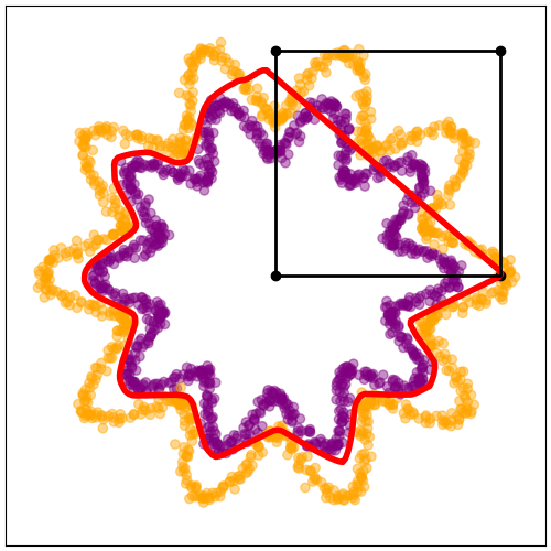
If we constrain the DNN to be affine on a specific region of its domain, it directly means that the decision boundary obtained by composing this constrained DNN with a linear classifier will also be linear within that region! Here is an illustration that is generated with the provided scripte, trying to solve a binary classification task of orange points versus purple with constrained region highlighted with the black dots and square:

Regression settings (Fig. 2 and 3, figure_2.py and figure_3.py)

Obviously the same goes if solving a regression task. We highlight here a simple example that consists of training a DNN solve a $\mathbb{R}^2 \mapsto \mathbb{R}$ regression problem where we use POLICE to impose the affine constraints on some part of the DNN's domain corresponding to Fig. 2:

Triangle region	Polygon region	(near) circle region

And we can also visualize the evolution during training that corresponds to Fig. 3:

Measuring computation times with different DNNs (Tab. 1, table_1.py)

To see that the proposed method is practical in many scenarios, we propose to see the required time to perform a forward+backward pass through a DNN for different input dimensions, widths and depths. Here are a few numbers that will be provided from the given code on a Quadro GP100:

Time (ms.) for input dim:784, width:128, depth:4

• unconstrained 1.34 $\pm$ 4.51
• POLICE: 8.31 $\pm$ 14.77
• slow-down factor: 6.2

Time (ms.) for input dim:2, width:512, depth:16

• unconstrained 3.01 $\pm$ 0.11
• POLICE: 30.72 $\pm$ 1.53
• slow-down factor: 10.2

Time (ms.) for input dim:3072, width:4096, depth:2

• unconstrained 23.85 $\pm$ 2.52
• POLICE: 91.54 $\pm$ 2.94
• slow-down factor: 3.8