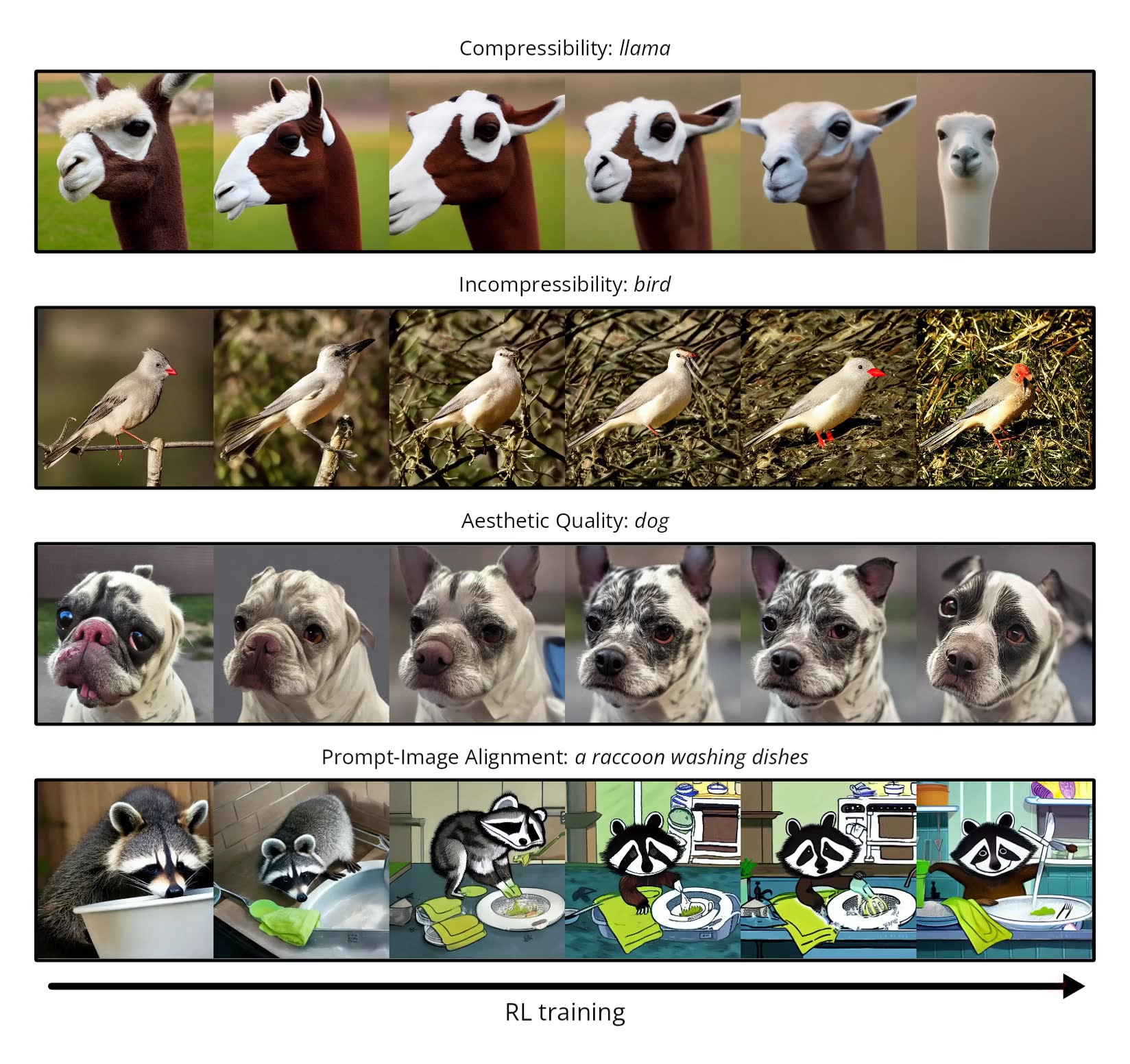
This is an implementation of Denoising Diffusion Policy Optimization (DDPO) in PyTorch with support for low-rank adaptation (LoRA). Unlike our original research code (which you can find here), this implementation runs on GPUs, and if LoRA is enabled, requires less than 10GB of GPU memory to finetune Stable Diffusion!
Requires Python 3.10 or newer.
git clone [email protected]:kvablack/ddpo-pytorch.git
cd ddpo-pytorch
pip install -e .accelerate launch scripts/train.pyThis will immediately start finetuning Stable Diffusion v1.5 for compressibility on all available GPUs using the config from config/base.py. It should work as long as each GPU has at least 10GB of memory. If you don't want to log into wandb, you can run wandb disabled before the above command.
Please note that the default hyperparameters in config/base.py are not meant to achieve good performance, they are just to get the code up and running as fast as possible. I would not expect to get good results without using a much larger number of samples per epoch and gradient accumulation steps.
A detailed explanation of all the hyperparameters can be found in config/base.py. Here are a few of the important ones.
At a high level, the problem of finetuning a diffusion model is defined by 2 things: a set of prompts to generate images, and a reward function to evaluate those images. The prompts are defined by a prompt_fn which takes no arguments and generates a random prompt each time it is called. The reward function is defined by a reward_fn which takes in a batch of images and returns a batch of rewards for those images. All of the prompt and reward functions currently implemented can be found in ddpo_pytorch/prompts.py and ddpo_pytorch/rewards.py, respectively.
Each DDPO epoch consists of generating a batch of images, computing their rewards, and then doing some training steps on those images. One important hyperparameter is the number of images generated per epoch; you want enough images to get a good estimate of the average reward and the policy gradient. Another important hyperparameter is the number of training steps per epoch.
However, these are not defined explicitly but are instead defined implicitly by several other hyperparameters. First note that all batch sizes are per GPU. Therefore, the total number of images generated per epoch is sample.batch_size * num_gpus * sample.num_batches_per_epoch. The effective total training batch size (if you include multi-GPU training and gradient accumulation) is train.batch_size * num_gpus * train.gradient_accumulation_steps. The number of training steps per epoch is the first number divided by the second number, or (sample.batch_size * sample.num_batches_per_epoch) / (train.batch_size * train.gradient_accumulation_steps).
(This assumes that train.num_inner_epochs == 1. If this is set to a higher number, then training will loop over the same batch of images multiple times before generating a new batch of images, and the number of training steps per epoch will be multiplied accordingly.)
At the beginning of each training run, the script will print out the calculated value for the number of images generated per epoch, the effective total training batch size, and the number of training steps per epoch. Make sure to double-check these numbers!
The image at the top of this README was generated using LoRA! However, I did use a fairly powerful DGX machine with 8xA100 GPUs, on which each experiment took about 4 hours for 100 epochs. In order to run the same experiments with a single small GPU, you would set sample.batch_size = train.batch_size = 1 and multiply sample.num_batches_per_epoch and train.gradient_accumulation_steps accordingly.
You can find the exact configs I used for the 4 experiments in config/dgx.py. For example, to run the aesthetic quality experiment:
accelerate launch scripts/train.py --config config/dgx.py:aestheticIf you want to run the LLaVA prompt-image alignment experiments, you need to dedicate a few GPUs to running LLaVA inference using this repo.


As you can see with the aesthetic experiment, if you run for long enough the algorithm eventually experiences instability. This might be remedied by decaying the learning rate. Interestingly, however, the actual qualitative samples you get after the instability are mostly fine -- the drop in the mean is caused by a few low-scoring outliers. This is clear from the full reward histogram, which you can see if you go to an individual run in wandb.

