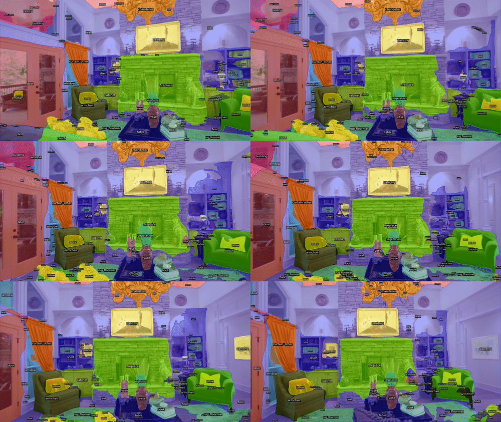
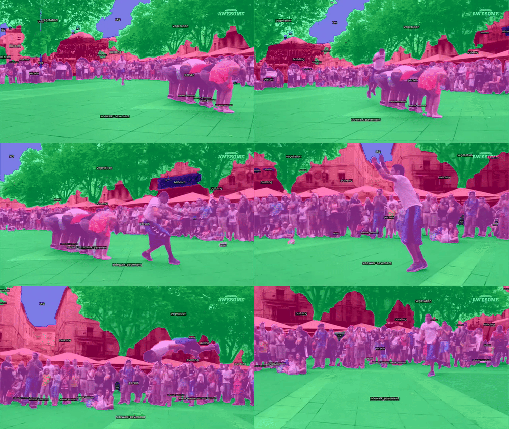
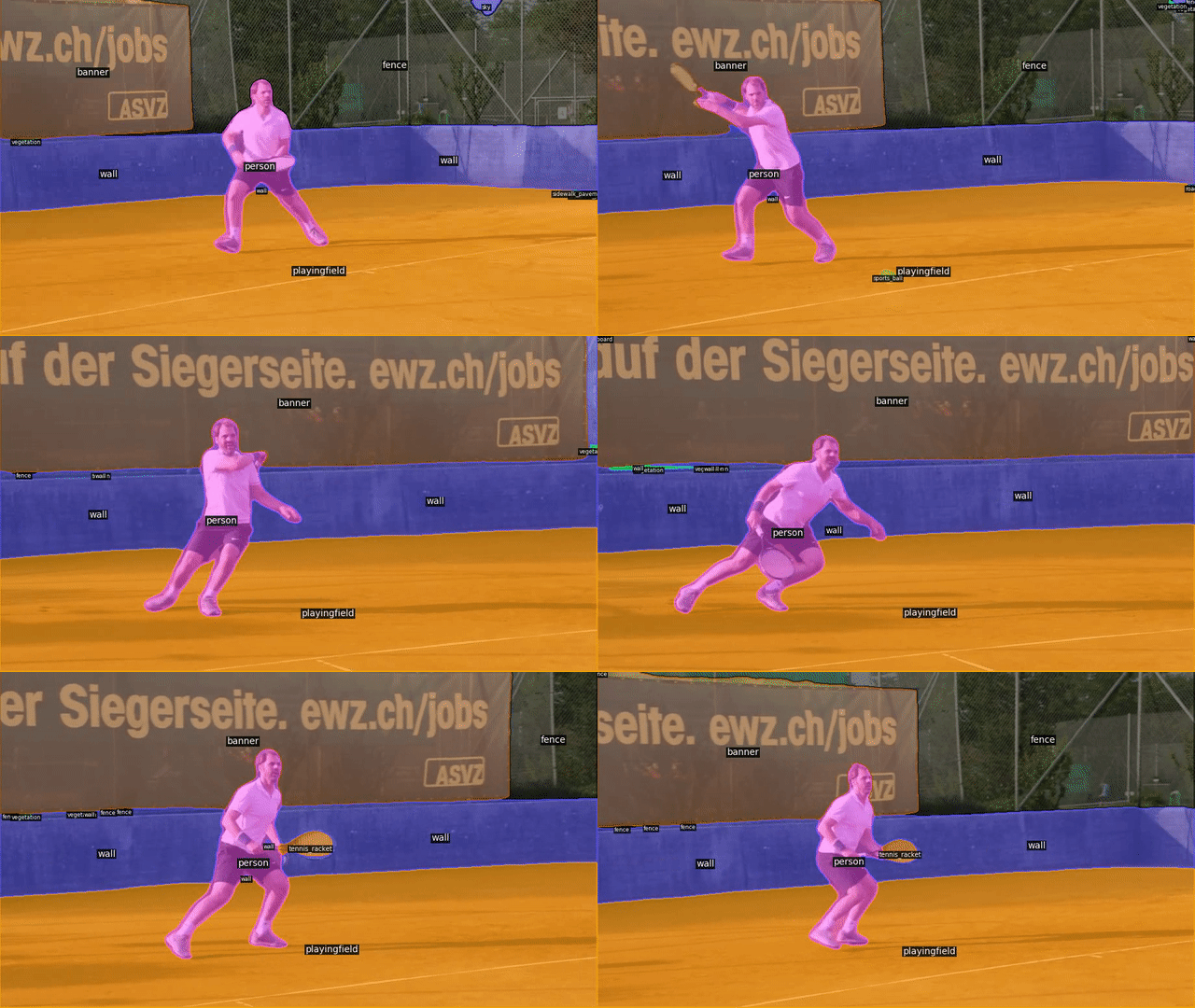
This repo includes the semantic segmentation pre-trained models, training and inference code for the paper:
MSeg: A Composite Dataset for Multi-domain Semantic Segmentation (CVPR 2020, Official Repo) [PDF]
John Lambert*,
Zhuang Liu*,
Ozan Sener,
James Hays,
Vladlen Koltun
Presented at CVPR 2020
This repo is the second of 4 repos that introduce our work. It provides utilities to train semantic segmentation models, using a HRNet-W48 or PSPNet backbone, sufficient to train a winning entry on the WildDash benchmark).
mseg-api: utilities to download the MSeg dataset, prepare the data on disk in a unified taxonomy, on-the-fly mapping to a unified taxonomy during training.
Two additional repos will be introduced in June 2020:
mseg-panoptic: provides Panoptic-FPN and Mask-RCNN training, based on Detectron2mseg-mturk: provides utilities to perform large-scale Mechanical Turk re-labeling
Install the mseg model from mseg-api
-
mseg_semanticcan be installed as a python package usingpip install -e /path_to_root_directory_of_the_repo/
Make sure that you can run import mseg_semantic in python, and you are good to go!
Each model is 528 MB in size. We provide download links and multi-scale testing results below:
Nicknames: VOC = PASCAL VOC, WD = WildDash, SN = ScanNet
| Model | Training Set | Training Taxonomy |
VOC mIoU |
PASCAL Context mIoU |
CamVid mIoU |
WD mIoU |
KITTI mIoU |
SN mIoU |
h. mean | Download Link |
|---|---|---|---|---|---|---|---|---|---|---|
| MSeg (1M) | MSeg train | Universal | 70.8 | 42.9 | 83.1 | 63.1 | 63.7 | 48.4 | 59.0 | Google Drive |
| MSeg (3M) | MSeg train | Universal | Google Drive |
Multi-scale inference greatly improves the smoothness of predictions, therefore our demos scripts use multi-scale config by default. While we train at 1080p, our predictions are often visually better when we feed in test images at 360p resolution.
If you have video input, and you would like to make predictions on each frame in the universal taxonomy, please set:
input_file=/path/to/my/video.mp4
If you have a set of images in a directory, and you would like to make a prediction in the universal taxonomy for each image, please set:
input_file=/path/to/my/directory
If you have as input a single image, and you would like to make a prediction in the universal taxonomy, please set:
input_file=/path/to/my/image
Now, run our demo script:
model_name=mseg-3m
model_path=/path/to/downloaded/model/from/google/drive
config=mseg_semantic/config/test/default_config_360.yaml
python -u mseg_semantic/tool/universal_demo.py \
  --config=${config} model_name ${model_name} model_path ${model_path} input_file ${input_file}
If you would like to make predictions in a specific dataset's taxonomy, e.g. Cityscapes, for the RVC Challenge, please run:
(will be added)
If you find this code useful for your research, please cite:
@InProceedings{MSeg_2020_CVPR,
author = {Lambert, John and Zhuang, Liu and Sener, Ozan and Hays, James and Koltun, Vladlen},
title = {{MSeg}: A Composite Dataset for Multi-domain Semantic Segmentation},
booktitle = {Computer Vision and Pattern Recognition (CVPR)},
year = {2020}
}
Many thanks to Hengshuang Zhao for his semseg repo, which we've based much of this repository off of.
Individually-trained models that serve as baselines:
Nicknames: VOC = PASCAL VOC, WD = WildDash, SN = ScanNet
| Model | Training Set | Training Taxonomy |
VOC mIoU |
PASCAL Context mIoU |
CamVid mIoU |
WD mIoU |
KITTI mIoU |
SN mIoU |
h. mean | Download Link |
|---|---|---|---|---|---|---|---|---|---|---|
| ADE20K (1M) | ADE20K train | Universal | 34.6 | 24.0 | 53.5 | 37.0 | 44.3 | 43.8 | 37.1 | Google Drive |
| BDD (1M) | BDD train | Universal | 13.5 | 6.9 | 71.0 | 52.1 | 55.0 | 1.4 | 6.1 | Google Drive |
| Cityscapes (1M ) | Cityscapes train | Universal | 12.1 | 6.5 | 65.3 | 30.1 | 58.1 | 1.7 | 6.7 | Google Drive |
| COCO (1M) | COCO train | Universal | 73.7 | 43.1 | 56.6 | 38.9 | 48.2 | 33.9 | 46.0 | Google Drive |
| IDD (1M) | IDD train | Universal | 14.5 | 6.3 | 70.5 | 40.6 | 50.7 | 1.6 | 6.5 | Google Drive |
| Mapillary (1M) | Mapillary train | Universal | 22.0 | 13.5 | 82.5 | 55.2 | 68.5 | 2.1 | 9.2 | Google Drive |
| SUN RGB-D (1M) | SUN RGBD train | Universal | 10.2 | 4.3 | 0.1 | 1.4 | 0.7 | 42.2 | 0.3 | Google Drive |
| Naive Mix Baseline (1M) | MSeg train. | Naive | Google Drive | |||||||
| Oracle (1M) | 77.0 | 46.0 | 79.1 | – | 57.5 | 62.2 | – | |||
| Oracle Model Download Links |
VOC2012 1M Model |
PASCAL Context 1M Model |
Camvid 1M Model |
N/A** | KITTI 1M Model |
ScanNet-20 1M Model |
-- | -- |
Note that the output number of classes for 7 of the models listed above will be identical (194 classes). These are the models that represent a single training dataset's performance -- ADE20K (1M), BDD (1M), Cityscapes (1M ), COCO (1M), IDD (1M), Mapillary (1M), SUN RGB-D (1M). When we train a baseline model on a single dataset, we train it in the universal taxonomy (w/ 194 classes). If we did not do so, we would need to specify 7*6=42 mappings (which would be unbelievably tedious and also fairly redundant) since we measure each's performance according to zero-shot cross-dataset generalization -- 7 training datasets with their own taxonomy, and each would need its own mapping to each of the 6 test sets.
By training each baseline that is trained on a single training dataset within the universal taxonomy, we are able to specify just 7+6=13 mappings in this table (each training dataset's taxonomy->universal taxonomy, and then universal taxonomy to each test dataset).
**WildDash has no training set, so an "oracle" model cannot be trained.
We use an HRNet-W48 backbone, we generally follow the recommendations of Zhao et al.: We use a ResNet50 or ResNet101 backbone, with a crop size of 713x713, with synchronized BN. All images are resized to 1080p at training time before a crop is taken.
Our data augmentation consists of random scaling in the range [0.5,2.0], random rotation in the range [-10,10] degrees. We use SGD with momentum 0.9, weight decay of 1e-4. We use a polynomial learning rate with power 0.9. Base learning rate is set to 1e-2. An auxiliary cross-entropy (CE) loss is added to intermediate activations, a linear combination with weight 0.4. In our data, we use 255 as an ignore/unlabeled flag for the CE loss. Logits are upsampled by a factor is 8 ("zoom factor") to match original label map resolution for loss calculation.
We use Pytorch's Distributed Data Parallel (DDP) package for multiprocessing, with the NCCL backend. Zhao et al. recommend a training batch size of 16, with different number of epochs per dataset (ADE20k: 200, Cityscapes: 200, Camvid: 100, VOC2012: 50). For inference, we use a multi-scale accumulation of probabilities: [0.5, 0.75, 1.0, 1.25, 1.5, 1.75]. Base size (ADE20K: 512, Camvid: 512, Cityscapes: 2048, VOC: 512) roughly equivalent to the average longer side of an image.
We use apex opt_level: 'O0'
For HRNet, we follow the original authors' suggestions: a learning rate of 0.01, momentum of 0.9, and weight decay of 5e-4. As above, we use a polynomial learning rate with power 0.9. Batch size is set to...
Download the HRNet Backbone Model here from the original authors' OneDrive.


