FACET is an open source library for human-explainable AI. It combines sophisticated model inspection and model-based simulation to enable better explanations of your supervised machine learning models.
FACET is composed of the following key components:
|
Model Inspection FACET introduces a new algorithm to quantify dependencies and interactions between features in ML models. This new tool for human-explainable AI adds a new, global perspective to the observation-level explanations provided by the popular SHAP approach. To learn more about FACET’s model inspection capabilities, see the getting started example below. |
|
Model Simulation FACET’s model simulation algorithms use ML models for virtual experiments to help identify scenarios that optimise predicted outcomes. To quantify the uncertainty in simulations, FACET utilises a range of bootstrapping algorithms including stationary and stratified bootstraps. For an example of FACET’s bootstrap simulations, see the quickstart example below. |
|
Enhanced Machine Learning Workflow FACET offers an efficient and transparent machine learning workflow, enhancing scikit-learn's tried and tested pipelining paradigm with new capabilities for model selection, inspection, and simulation. FACET also introduces sklearndf [documentation] an augmented version of scikit-learn with enhanced support for pandas data frames that ensures end-to-end traceability of features. |
FACET supports both PyPI and Anaconda.
conda install gamma-facet -c bcg_gamma -c conda-forgepip install gamma-facetThe following quickstart guide provides a minimal example workflow to get you up and running with FACET. For additional tutorials and the API reference, see the FACET documentation.
Changes and additions to new versions are summarized in the release notes.
To demonstrate the model inspection capability of FACET, we first create a pipeline to fit a learner. In this simple example we will use the diabetes dataset which contains age, sex, BMI and blood pressure along with 6 blood serum measurements as features. This dataset was used in this publication. A transformed version of this dataset is also available on scikit-learn here.
In this quickstart we will train a Random Forest regressor using 10 repeated 5-fold CV to predict disease progression after one year. With the use of sklearndf we can create a pandas DataFrame compatible workflow. However, FACET provides additional enhancements to keep track of our feature matrix and target vector using a sample object (Sample) and easily compare hyperparameter configurations and even multiple learners with the LearnerRanker.
# standard imports
import pandas as pd
from sklearn.model_selection import RepeatedKFold

# some helpful imports from sklearndf
from sklearndf.pipeline import RegressorPipelineDF
from sklearndf.regression import RandomForestRegressorDF

# relevant FACET imports
from facet.data import Sample
from facet.selection import LearnerRanker, LearnerGrid

# declaring url with data
data_url = 'https://web.stanford.edu/~hastie/Papers/LARS/diabetes.data'

#importing data from url
diabetes_df = pd.read_csv(data_url, delimiter='\t').rename(
    # renaming columns for better readability
    columns={
        'S1': 'TC', # total serum cholesterol
        'S2': 'LDL', # low-density lipoproteins
        'S3': 'HDL', # high-density lipoproteins
        'S4': 'TCH', # total cholesterol/ HDL
        'S5': 'LTG', # lamotrigine level
        'S6': 'GLU', # blood sugar level
        'Y': 'Disease_progression' # measure of progress since 1yr of baseline
    }
)

# create FACET sample object
diabetes_sample = Sample(observations=diabetes_df, target_name="Disease_progression")

# create a (trivial) pipeline for a random forest regressor
rnd_forest_reg = RegressorPipelineDF(
    regressor=RandomForestRegressorDF(n_estimators=200, random_state=42)
)

# define grid of models which are "competing" against each other
rnd_forest_grid = [
    LearnerGrid(
        pipeline=rnd_forest_reg,
        learner_parameters={
            "min_samples_leaf": [8, 11, 15],
            "max_depth": [4, 5, 6],
        }
    ),
]

# create repeated k-fold CV iterator
rkf_cv = RepeatedKFold(n_splits=5, n_repeats=10, random_state=42)

# rank your candidate models by performance (default is mean CV score - 2*SD)
ranker = LearnerRanker(
    grids=rnd_forest_grid, cv=rkf_cv, n_jobs=-3
).fit(sample=diabetes_sample)

# get summary report
ranker.summary_report()
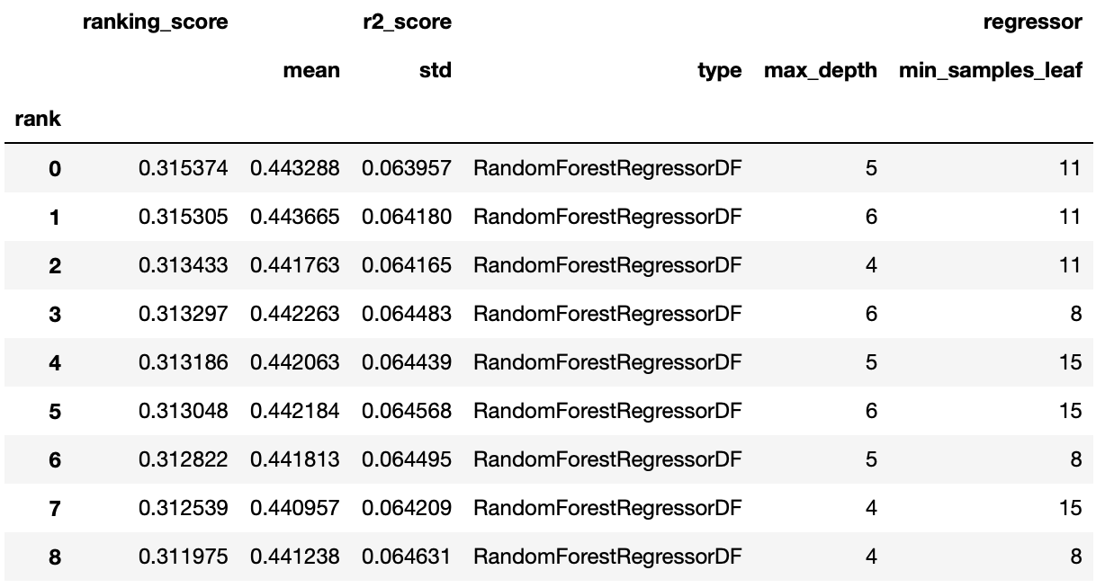
We can see based on this minimal workflow that a value of 11 for minimum samples in the leaf and 5 for maximum tree depth was the best performing of the three considered values. This approach easily extends to additional hyperparameters for the learner, and for multiple learners.
FACET implements several model inspection methods for scikit-learn estimators. FACET enhances model inspection by providing global metrics that complement the local perspective of SHAP (see [arXiv:2107.12436] for a formal description).
The key global metrics for each pair of features in a model are:
Synergy
The degree to which the model combines information from one feature with another to predict the target. For example, let's assume we are predicting cardiovascular health using age and gender and the fitted model includes a complex interaction between them. This means these two features are synergistic for predicting cardiovascular health. Further, both features are important to the model and removing either one would significantly impact performance. Let's assume age brings more information to the joint contribution than gender. This asymmetric contribution means the synergy for (age, gender) is less than the synergy for (gender, age). To think about it another way, imagine the prediction is a coordinate you are trying to reach. From your starting point, age gets you much closer to this point than gender, however, you need both to get there. Synergy reflects the fact that gender gets more help from age (higher synergy from the perspective of gender) than age does from gender (lower synergy from the perspective of age) to reach the prediction. This leads to an important point: synergy is a naturally asymmetric property of the global information two interacting features contribute to the model predictions. Synergy is expressed as a percentage ranging from 0% (full autonomy) to 100% (full synergy).
Redundancy
The degree to which a feature in a model duplicates the information of a second feature to predict the target. For example, let's assume we had house size and number of bedrooms for predicting house price. These features capture similar information as the more bedrooms the larger the house and likely a higher price on average. The redundancy for (number of bedrooms, house size) will be greater than the redundancy for (house size, number of bedrooms). This is because house size "knows" more of what number of bedrooms does for predicting house price than vice-versa. Hence, there is greater redundancy from the perspective of number of bedrooms. Another way to think about it is removing house size will be more detrimental to model performance than removing number of bedrooms, as house size can better compensate for the absence of number of bedrooms. This also implies that house size would be a more important feature than number of bedrooms in the model. The important point here is that like synergy, redundancy is a naturally asymmetric property of the global information feature pairs have for predicting an outcome. Redundancy is expressed as a percentage ranging from 0% (full uniqueness) to 100% (full redundancy).
# fit the model inspector
from facet.inspection import LearnerInspector
inspector = LearnerInspector(n_jobs=-3)
inspector.fit(crossfit=ranker.best_model_crossfit_)
Synergy
# visualise synergy as a matrix
from pytools.viz.matrix import MatrixDrawer
synergy_matrix = inspector.feature_synergy_matrix()
MatrixDrawer(style="matplot%").draw(synergy_matrix, title="Synergy Matrix")
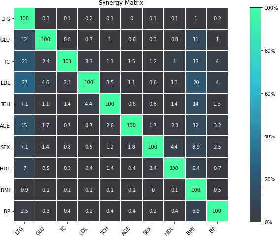
For any feature pair (A, B), the first feature (A) is the row, and the second feature (B) the column. For example, looking across the row for LTG (Lamotrigine) there is hardly any synergy with other features in the model (≤ 1%). However, looking down the column for LTG (i.e., from the perspective of other features relative with LTG) we find that many features (the rows) are aided by synergy with with LTG (up to 27% in the case of LDL). We conclude that:
- LTG is a strongly autonomous feature, displaying minimal synergy with other features for predicting disease progression after one year.
- The contribution of other features to predicting disease progression after one year is partly enabled by the presence of LTG.
High synergy between pairs of features must be considered carefully when investigating impact, as the values of both features jointly determine the outcome. It would not make much sense to consider LDL without the context provided by LTG given close to 27% synergy of LDL with LTG for predicting progression after one year.
Redundancy
# visualise redundancy as a matrix
redundancy_matrix = inspector.feature_redundancy_matrix()
MatrixDrawer(style="matplot%").draw(redundancy_matrix, title="Redundancy Matrix")
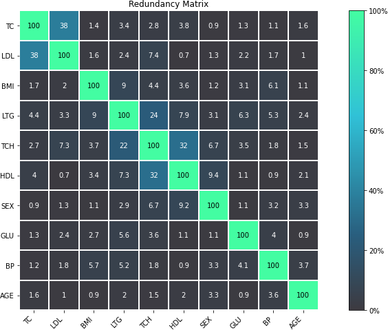
For any feature pair (A, B), the first feature (A) is the row, and the second feature (B) the column. For example, if we look at the feature pair (LDL, TC) from the perspective of LDL (Low-Density Lipoproteins), then we look-up the row for LDL and the column for TC and find 38% redundancy. This means that 38% of the information in LDL to predict disease progression is duplicated in TC. This redundancy is the same when looking "from the perspective" of TC for (TC, LDL), but need not be symmetrical in all cases (see LTG vs. TCH).
If we look at TCH, it has between 22–32% redundancy each with LTG and HDL, but the same does not hold between LTG and HDL – meaning TCH shares different information with each of the two features.
Clustering redundancy
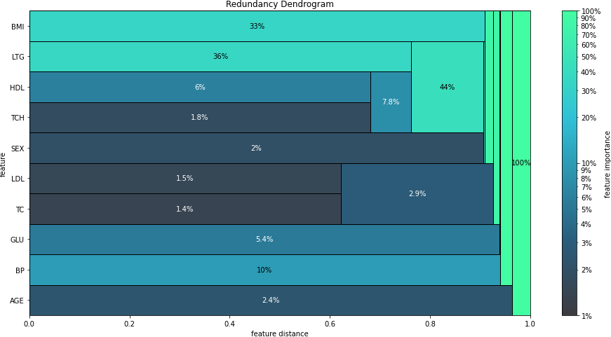
As detailed above redundancy and synergy for a feature pair is from the "perspective" of one of the features in the pair, and so yields two distinct values. However, a symmetric version can also be computed that provides not only a simplified perspective but allows the use of (1 - metric) as a feature distance. With this distance hierarchical, single linkage clustering is applied to create a dendrogram visualization. This helps to identify groups of low distance, features which activate "in tandem" to predict the outcome. Such information can then be used to either reduce clusters of highly redundant features to a subset or highlight clusters of highly synergistic features that should always be considered together.
Let's look at the example for redundancy.
# visualise redundancy using a dendrogram
from pytools.viz.dendrogram import DendrogramDrawer
redundancy = inspector.feature_redundancy_linkage()
DendrogramDrawer().draw(data=redundancy, title="Redundancy Dendrogram")
Based on the dendrogram we can see that the feature pairs (LDL, TC) and (HDL, TCH) each represent a cluster in the dendrogram and that LTG and BMI have the highest importance. As potential next actions we could explore the impact of removing TCH, and one of TC or LDL to further simplify the model and obtain a reduced set of independent features.
Please see the API reference for more detail.
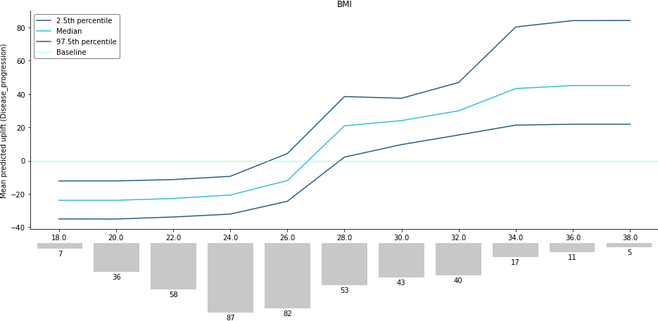
Taking the BMI feature as an example of an important and highly independent feature, we do the following for the simulation:
- We use FACET's ContinuousRangePartitioner to split the range of observed values of BMI into intervals of equal size. Each partition is represented by the central value of that partition.
- For each partition, the simulator creates an artificial copy of the original sample assuming the variable to be simulated has the same value across all observations – which is the value representing the partition. Using the best LearnerCrossfit acquired from the ranker, the simulator now re-predicts all targets using the models trained for all folds and determines the average uplift of the target variable resulting from this.
- The FACET SimulationDrawer allows us to visualise the result; both in a matplotlib and a plain-text style.
Finally, because FACET can use bootstrap cross validation, we can create a crossfit from our previous LearnerRanker best model to perform the simulation, so we can quantify the uncertainty by using bootstrap confidence intervals.
# FACET imports
from facet.validation import BootstrapCV
from facet.crossfit import LearnerCrossfit
from facet.simulation import UnivariateUpliftSimulator
from facet.data.partition import ContinuousRangePartitioner
from facet.simulation.viz import SimulationDrawer

# create bootstrap CV iterator
bscv = BootstrapCV(n_splits=1000, random_state=42)

# create a bootstrap CV crossfit for simulation using best model
boot_crossfit = LearnerCrossfit(
    pipeline=ranker.best_model_,
    cv=bscv,
    n_jobs=-3,
    verbose=False,
).fit(sample=diabetes_sample)

SIM_FEAT = "BMI"
simulator = UnivariateUpliftSimulator(crossfit=boot_crossfit, n_jobs=-3)

# split the simulation range into equal sized partitions
partitioner = ContinuousRangePartitioner()

# run the simulation
simulation = simulator.simulate_feature(feature_name=SIM_FEAT, partitioner=partitioner)

# visualise results
SimulationDrawer().draw(data=simulation, title=SIM_FEAT)
We would conclude from the figure that higher values of BMI are associated with an increase in disease progression after one year, and that for a BMI of 28 and above, there is a significant increase in disease progression after one year of at least 26 points.
FACET is stable and is being supported long-term.
Contributions to FACET are welcome and appreciated. For any bug reports or feature requests/enhancements please use the appropriate GitHub form, and if you wish to do so, please open a PR addressing the issue.
We do ask that for any major changes please discuss these with us first via an issue or using our team email: [email protected].
For further information on contributing please see our contribution guide.
FACET is licensed under Apache 2.0 as described in the LICENSE file.
FACET is built on top of two popular packages for Machine Learning:
- The scikit-learn learners and pipelining make up implementation of the underlying algorithms. Moreover, we tried to design the FACET API to align with the scikit-learn API.
- The SHAP implementation is used to estimate the shapley vectors which FACET then decomposes into synergy, redundancy, and independence vectors.
If you would like to know more about the team behind FACET please see the about us page.
We are always on the lookout for passionate and talented data scientists to join the BCG GAMMA team. If you would like to know more you can find out about BCG GAMMA, or have a look at career opportunities.
