%%%%%%%%%%%%%%%%%%%%%%%%%%%
Frequency_of_operation = 77e9;
Max_Range = 200;
Range_Resolution = 1;
Max_Velocity = 100;
%%%%%%%%%%%%%%%%%%%%%%%%%%%

speed_of_light = 3e8;


fc= 77e9;             %carrier freq
sweep_time_factor = 5.5;

B      = speed_of_light / (2 * Range_Resolution); % Bandwidth of the FMCW, Bsweep
Tchirp = (sweep_time_factor*2*Max_Range)/speed_of_light; % Chirp Time of the FMCW
slope = B/Tchirp; %slope of the FMCW  

R = 100;         %initial position 
v = 50;        %initial velocity

%The number of chirps in one sequence. Its ideal to have 2^ value for the ease of running the FFT
%for Doppler Estimation. 
Nd=128;                   % #of doppler cells OR #of sent periods % number of chirps

%The number of samples on each chirp. 
Nr=1024;                  %for length of time OR # of range cells

% Timestamp for running the displacement scenario for every sample on each
% chirp
t=linspace(0,Nd*Tchirp,Nr*Nd); %total time for samples


%Creating the vectors for Tx, Rx and Mix based on the total samples input.
Tx=zeros(1,length(t)); %transmitted signal
Rx=zeros(1,length(t)); %received signal
Mix = zeros(1,length(t)); %beat signal

%Similar vectors for range_covered and time delay.
r_t=zeros(1,length(t));
td=zeros(1,length(t));

Mix = reshape(Mix,[Nr,Nd]);

 % *%TODO* :
%run the FFT on the beat signal along the range bins dimension (Nr) and
%normalize.
sig_fft = fft(Mix,Nr);  
sig_fft = sig_fft./Nr;

% *%TODO* :
% Take the absolute value of FFT output
sig_fft = abs(sig_fft);  

 % *%TODO* :
% Output of FFT is double sided signal, but we are interested in only one side of the spectrum.
% Hence we throw out half of the samples.
single_side_sig_fft = sig_fft(1:Nr/2);


%plotting the range
figure ('Name','Range from First FFT')
subplot(2,1,1)

% *%TODO* :
% plot FFT output 
plot(single_side_sig_fft); 

Mix=reshape(Mix,[Nr,Nd]);

% 2D FFT using the FFT size for both dimensions.
sig_fft2 = fft2(Mix,Nr,Nd);

% Taking just one side of signal from Range dimension.
sig_fft2 = sig_fft2(1:Nr/2,1:Nd);
sig_fft2 = fftshift (sig_fft2);
RDM = abs(sig_fft2);
RDM = 10*log10(RDM) ;

%use the surf function to plot the output of 2DFFT and to show axis in both
%dimensions
doppler_axis = linspace(-100,100,Nd);
range_axis = linspace(-200,200,Nr/2)*((Nr/2)/400);
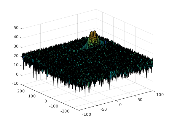
figure,surf(doppler_axis,range_axis,RDM);

Tcr = 10;      %the number of Training Cells in both the dimensions.
Tcd = 4;

Gcr = 4;       %the number of Guard Cells in both dimensions around the 
Gcd = 4;       %Cell under test (CUT) for accurate estimation
      
offset = 1.4;  % offset the threshold by SNR value in dB

RDM = RDM/max(max(RDM));

for i = Tr+Gr+1:(Nr/2)-(Gr+Tr)
    for j = Td+Gd+1:Nd-(Gd+Td)
        
       % Create a vector to store noise_level for each iteration on training cells
        noise_level = zeros(1,1);
        
        % Calculate noise SUM in the area around CUT
        for p = i-(Tr+Gr) : i+(Tr+Gr)
            for q = j-(Td+Gd) : j+(Td+Gd)
                if (abs(i-p) > Gr || abs(j-q) > Gd)
                    noise_level = noise_level + db2pow(RDM(p,q));
                end
            end
        end

% Calculate threshould from noise average then add the offset
        threshold = pow2db(noise_level/(2*(Td+Gd+1)*2*(Tr+Gr+1)-(Gr*Gd)-1));
        threshold = threshold + offset;
        CUT = RDM(i,j);
        
        if (CUT < threshold)
            RDM(i,j) = 0;
        else
            RDM(i,j) = 1;
        end
    end
end

RDM(union(1:(Tr+Gr),end-(Tr+Gr-1):end),:) = 0;  % Rows
RDM(:,union(1:(Td+Gd),end-(Td+Gd-1):end)) = 0;  % Columns 

figure('Name','CA-CFAR Filtered RDM')
surf(doppler_axis,range_axis,RDM);
colorbar;